Heating Adobe Houses

The thicker the adobe walls are, the better, as it will maintain a nearly constant inside temperature. However, it would also be more expensive to build. Here, we try to model the heat flow through adobe walls using the heat equation to find the optimum wall thickness.

import numpy as np
import matplotlib.pyplot as plt
from time import time
import numba
from numba import jit, cuda

K0 = 273.15 # 0 Celsius in Kelvin

Here, we have use synthetic data to approximate the typical diurnal temperature variation in these climatic regions.

@numba.jit("f8(f8)", nopython=True, nogil=True, fastmath = True)
def external_temperature(sec):
    h = sec/3600
    h = h%24
    t = 15*np.sin(np.pi*h/12 + 3.9) + 24
    return K0 + t

Defining the problem

alpha = 0.27
days = 7
duration = 3600*24*days #seconds
nodes = 300

# initialize wall temperature as a gradient
# where initial inner wall is set at 25 degree Celsius
wall = np.linspace(external_temperature(0), 25+K0, nodes) 

Solving the heat equation

@numba.jit("(f8[:],f8,f8,f8)", nopython=True, nogil=True, fastmath = True, cache=True)
def solve_heat_eqn(init_state, duration, dt, dx):
    wall = init_state.copy()
    counter = 0
    
    inners = []
    
    while counter < duration :
        w = wall.copy()
        for i in range(1, nodes - 1):

            wall[i] = dt * alpha * (w[i - 1] - 2 * w[i] + w[i + 1]) / dx ** 2 + w[i]

        counter += dt
        wall[0] = external_temperature(counter)
        wall[-1] = wall[-2]
        
        inners.append(wall[-1])
        
    return wall, np.array(inners)

External temperature for reference

def external_temperature_hour(h):
    h = h%24
    t = 15*np.sin(np.pi*h/12 + 3.9) + 24
    return t
hours_xs = np.linspace(0, 24*days, 300)

Solve heat equation for different wall thicknesses

def get_inner_temperatures(thickness):
    
    dx = thickness / (nodes-1)
    dt = 0.5 * dx**2 / alpha

    start = time()
    print(f'For t = {thickness} mm:\n  Iterations: {duration/dt:.0f}\n  dt = {dt:.3f} s')
    final, inners = solve_heat_eqn(wall, duration, dt, dx)
    end = time()
    print(f'  Time elapsed: {end - start:.3f} s\n')
    
    N = len(inners)
    if N > 1e5:
        k = int(N//1e5)
        inners = inners[::k]
        
    return inners   

thicknesses = {150:[], 120:[], 100:[], 200:[]}
for thickness in thicknesses:
    thicknesses[thickness] = get_inner_temperatures(thickness)

For t = 150 mm:
  Iterations: 1297673
  dt = 0.466 s
  Time elapsed: 0.575 s

For t = 120 mm:
  Iterations: 2027615
  dt = 0.298 s
  Time elapsed: 0.924 s

For t = 100 mm:
  Iterations: 2919765
  dt = 0.207 s
  Time elapsed: 1.333 s

For t = 200 mm:
  Iterations: 729941
  dt = 0.829 s
  Time elapsed: 0.330 s

Plotting inner temperatures

variations = {}

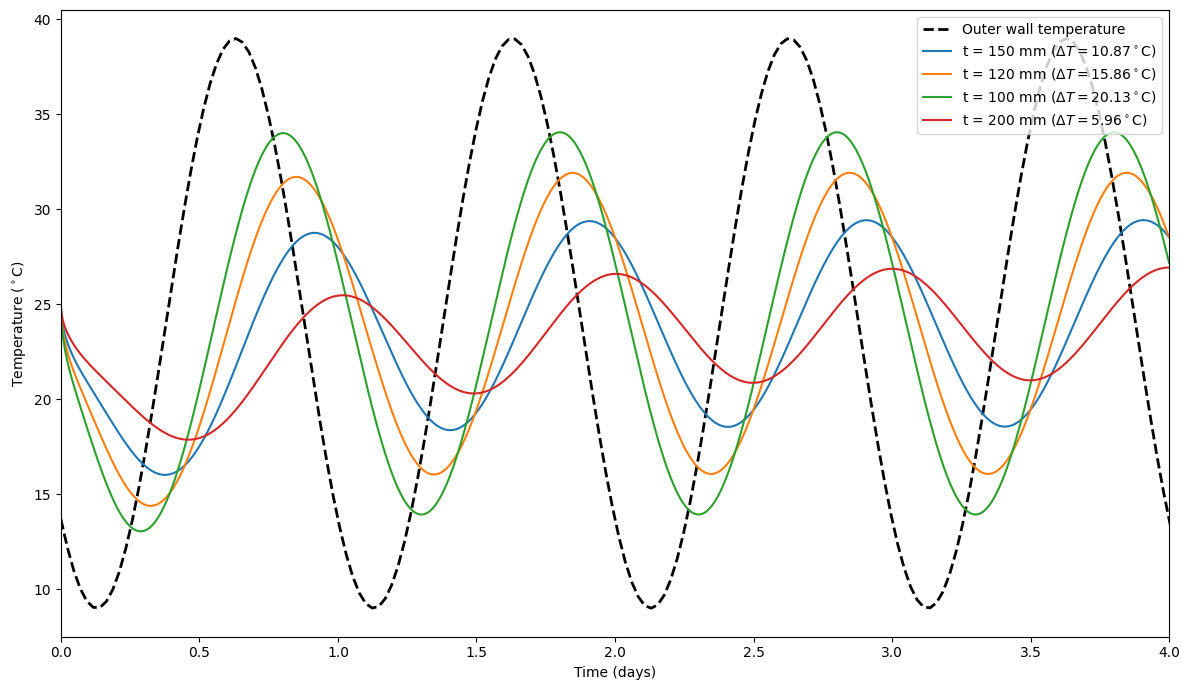
plt.figure(figsize=(12,7))
plt.plot(hours_xs/24, external_temperature_hour(hours_xs), 'k--', label='Outer wall temperature', alpha=1, linewidth=2)

for thickness in thicknesses:
    inner_temps = thicknesses[thickness]-K0
    xss = np.linspace(0, duration/3600, len(inner_temps))
    
    stable_region = int(len(inner_temps)/2)
    maxT = np.max(inner_temps[stable_region:])
    minT = np.min(inner_temps[stable_region:])
    print(f'Temperature variation: {minT:.2f} to {maxT:.2f} Celsius ({maxT-minT:.2f})')
    
    variations[thickness] = maxT-minT
    plt.plot(xss/24, inner_temps, label=f't = {thickness} mm ('+r"$\Delta T =$"+f'{round(maxT-minT,2)}'+r"$^\circ$C)")
    
plt.ylabel(r'Temperature ($^\circ$C)')
plt.xlabel('Time (days)')
plt.xlim(0,4)
plt.legend(loc='upper right')
plt.tight_layout()
plt.savefig('plots/4/var0.png', dpi=200)

Temperature variation: 18.56 to 29.44 Celsius (10.87)
Temperature variation: 16.07 to 31.93 Celsius (15.86)
Temperature variation: 13.94 to 34.06 Celsius (20.13)
Temperature variation: 21.00 to 26.96 Celsius (5.96)

Narrow down the temperature range

thicknesses = {180:[], 190:[], 200:[], 210:[], 220:[]}
for thickness in thicknesses:
    thicknesses[thickness] = get_inner_temperatures(thickness)

For t = 180 mm:
  Iterations: 901162
  dt = 0.671 s
  Time elapsed: 0.413 s

For t = 190 mm:
  Iterations: 808799
  dt = 0.748 s
  Time elapsed: 0.360 s

For t = 200 mm:
  Iterations: 729941
  dt = 0.829 s
  Time elapsed: 0.324 s

For t = 210 mm:
  Iterations: 662078
  dt = 0.913 s
  Time elapsed: 0.298 s

For t = 220 mm:
  Iterations: 603257
  dt = 1.003 s
  Time elapsed: 0.271 s

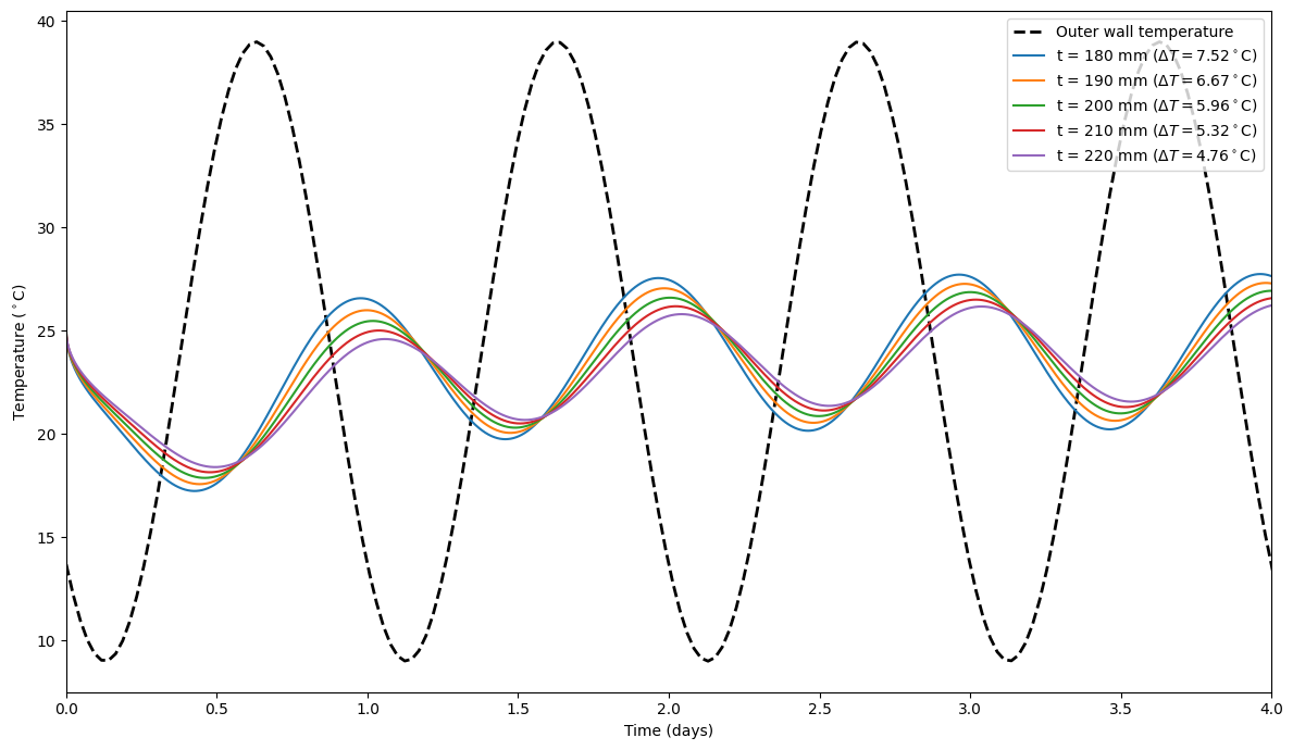
plt.figure(figsize=(12,7))
plt.plot(hours_xs/24, external_temperature_hour(hours_xs), 'k--', label='Outer wall temperature', alpha=1, linewidth=2)

for thickness in thicknesses:
    inner_temps = thicknesses[thickness]-K0
    xss = np.linspace(0, duration/3600, len(inner_temps))
    
    stable_region = int(len(inner_temps)/2)
    maxT = np.max(inner_temps[stable_region:])
    minT = np.min(inner_temps[stable_region:])
    print(f'Temperature variation: {minT:.2f} to {maxT:.2f} Celsius ({maxT-minT:.2f})')
    
    variations[thickness] = maxT-minT
    plt.plot(xss/24, inner_temps, label=f't = {thickness} mm ('+r"$\Delta T =$"+f'{round(maxT-minT,2)}'+r"$^\circ$C)")
    
plt.ylabel(r'Temperature ($^\circ$C)')
plt.xlabel('Time (days)')
plt.xlim(0,4)
plt.legend(loc='upper right')
plt.tight_layout()
plt.savefig('plots/4/var1.png', dpi=200)

Temperature variation: 20.24 to 27.76 Celsius (7.52)
Temperature variation: 20.66 to 27.33 Celsius (6.67)
Temperature variation: 21.00 to 26.96 Celsius (5.96)
Temperature variation: 21.31 to 26.63 Celsius (5.32)
Temperature variation: 21.57 to 26.34 Celsius (4.76)

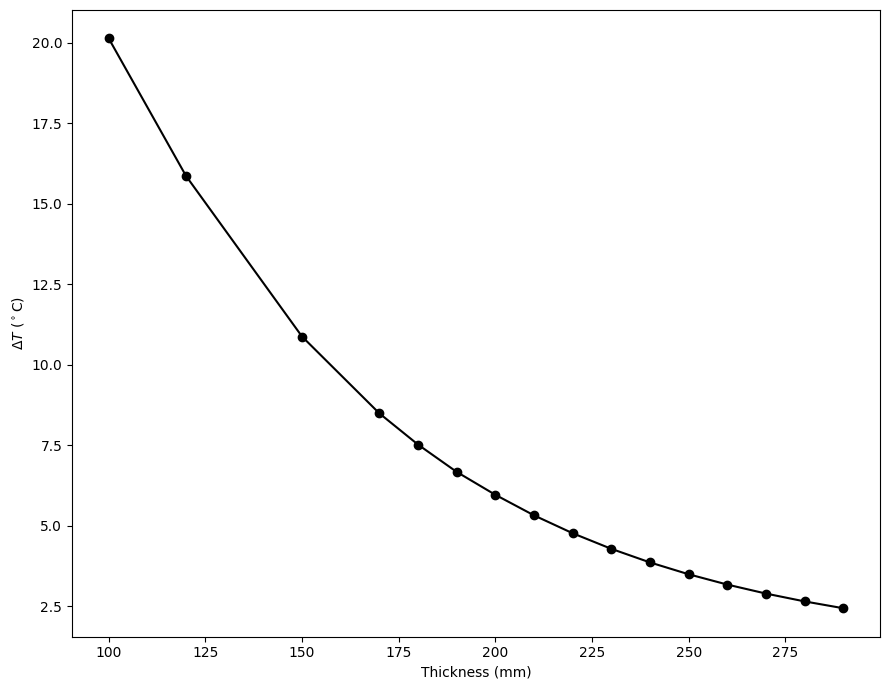
\(\Delta T\) vs Thickness

As we can see that the temperature variations around 200 mm get close to the human comfort range. Let us now plot \(\Delta T\) vs thickness.

thicknesses = [T for T in range(170, 300, 10)]
for thickness in thicknesses:
    inner_temps = get_inner_temperatures(thickness)
    stable_region = int(len(inner_temps)/2)
    maxT = np.max(inner_temps[stable_region:])
    minT = np.min(inner_temps[stable_region:])
    
    variations[thickness] = maxT-minT

For t = 170 mm:
  Iterations: 1010299
  dt = 0.599 s
  Time elapsed: 0.456 s

For t = 180 mm:
  Iterations: 901162
  dt = 0.671 s
  Time elapsed: 0.402 s

For t = 190 mm:
  Iterations: 808799
  dt = 0.748 s
  Time elapsed: 0.360 s

For t = 200 mm:
  Iterations: 729941
  dt = 0.829 s
  Time elapsed: 0.325 s

For t = 210 mm:
  Iterations: 662078
  dt = 0.913 s
  Time elapsed: 0.295 s

For t = 220 mm:
  Iterations: 603257
  dt = 1.003 s
  Time elapsed: 0.270 s

For t = 230 mm:
  Iterations: 551940
  dt = 1.096 s
  Time elapsed: 0.247 s

For t = 240 mm:
  Iterations: 506904
  dt = 1.193 s
  Time elapsed: 0.227 s

For t = 250 mm:
  Iterations: 467162
  dt = 1.295 s
  Time elapsed: 0.207 s

For t = 260 mm:
  Iterations: 431918
  dt = 1.400 s
  Time elapsed: 0.189 s

For t = 270 mm:
  Iterations: 400516
  dt = 1.510 s
  Time elapsed: 0.177 s

For t = 280 mm:
  Iterations: 372419
  dt = 1.624 s
  Time elapsed: 0.164 s

For t = 290 mm:
  Iterations: 347178
  dt = 1.742 s
  Time elapsed: 0.153 s

plt.figure(figsize=(9,7))
variations = dict(sorted(variations.items()))
plt.plot(variations.keys(), variations.values(), '-ko')
plt.ylabel(r'$\Delta T$ ($^\circ$C)')
plt.xlabel('Thickness (mm)') 
plt.tight_layout()
plt.savefig('plots/4/var_fin.png', dpi=200)