Sample-Based Guided Quantum Walk

A Non-Variational Algorithm for Combinatorial Optimization. Based on Nzongani, U. et al., (2025).

Alert: Make sure all necessary python packages are installed.

!pip install networkx

# essentials
import networkx as nx
import numpy as np
from numba import njit
import numpy as np
import scipy.sparse as sp
from qiskit import QuantumRegister, ClassicalRegister, QuantumCircuit, transpile
from qiskit.quantum_info import Statevector
from qiskit.visualization import plot_histogram
from qiskit_aer.primitives import SamplerV2

# data analysis
from functools import partial
import numbers
from collections import defaultdict
from scipy.interpolate import interp1d
import random
from typing import List, Set
from itertools import combinations
from tqdm import tqdm
from collections import Counter

# plotting tools
import matplotlib.pyplot as plt
import matplotlib.cm as cm
import matplotlib.colors as colors
from matplotlib.lines import Line2D
import matplotlib.patches as mpatches
from matplotlib.legend_handler import HandlerTuple
from mpl_toolkits.axes_grid1.inset_locator import inset_axes
import scienceplots
plt.style.use(['science', 'notebook', 'no-latex'])

Introduction¶

Combinatorial optimization problems involve finding the best, or “optimal” solution from a finite set of discrete possibilities, often in vast search spaces.
On a Classical Computer, generally for a combinatorial optimization problem with $n$ inputs, the solution space is often exponential, i.e. $2^n$ in size. Especially NP-hard problems (problems that have no known algorithm to solve it in $O(n^k)$ ), the only way is to use brute force.
On the other hand, we can use quantum algorithms, which are much better suited to explore massive solution spaces than classical computers. Just $n$ qubits can be used to represent the candidate space as a $2^n$ -dimensional Hilbert space $H^{⊗n}$ . Hence, the runtime will scale polynomially, instead of exponentially, w.r.t. the input size.

Formulating the problem¶

Every optimization problem can be represented by a cost function, which maps each possible solution to the quality of the solution, least cost meaning the highest quality and vice-versa.

Hence, we essentially have tp solve optimization problems of the form,

\vec{x}^* = \min_{\vec{x}\in\{0,1\}^n} \, \left\{C(\vec{x}) \textrm{ such that } \vec{x} \in \mathcal{F}\right\}

where

$C:\{0,1\}^n \rightarrow \mathbb{R} \equiv$ cost function,
$\mathcal{F} \equiv$ the constraint set (i.e = feasible solutions, which satisfy the constraints),
$\vec{x}^* \equiv$ optimal solution. The optimal solution has the least value of cost function.

We call any $\vec{x} \in \mathcal{F}$ a feasible decision (i.e., any binary decision that respects the constraints). If $x$ is a feasible decision, then an $\vec{\epsilon}$ -approximate solution ( $\vec{\epsilon}>0$ ), such that,

C(\vec{x}) - C(\vec{x^*}) \leq \epsilon

(1)

Quantum Walk Implementation¶

Let us see how to solve a combinatorial optimization problem using quantum adiabatic evolution. (Albash & Lidar, 2018).

Traditional adiabatic evolution states that if the system starts in the ground state of $H_0$ and evolves slowly enough, it will remain in the ground state of $H(t)$ during the evolution. Eventually, it will end up in the ground state of $H_1$ when $t=T$ .

In our case, we can choose our Hamiltonians such that the ground state of $H_0$ is easy to prepare and that of $H_1$ encodes the solution of a combinatorial optimization problem -- an adiabatic evolution would lead to the optimal solution.

H(t)=\left(1-\frac{t}{T}\right)H_0 + \frac{t}{T}H_1.

Guided Quantum Walk¶

GQWs generalize adiabatic evolution by using a time-dependent hopping rate, $\Gamma(t)$ (Schulz et. al., 2024),

H(t)=\Gamma(t)\,H_M + H_C.

where $H_M$ is the mixer hamiltonian, which prepares the superposition of all possible solutions and $H_C$ is the cost Hamiltonian which factors in the cost function and guides the state to the optimal solution.

To maximize amplitude transfer toward optimal solutions, the energy levels of $\Gamma(t)H_M$ and $H_C$ must be balanced. The solution space can be represented as a hypercube. An edge exists between vertices $j$ and $k$ only if they differ by exactly one bit.

$\left|\Delta^M_{jk}\right|$ is the difference between 2 consecutive levels (since $j$ and $j$ adjacent in the initial state). This is the minimal energy required to move amplitude from one ‘shell’ of the hypercube to the next. Only for $|\Gamma \Delta_{jk}^M|\approx \Delta_{jk}^C$ the two Hamiltonians’ relative strengths are balanced. Thus, amplitude transfers can only occur efficiently among specific subsets of vertex pairs with approximately this energy gap, this is known as the balancing condition. Any imbalance, or one of the terms will dominate the other.

Aim of the Paper¶

The SamBa-GQW algorithm is based on the idea is that one does not need to have the exact spectrum of $H_C$ nor optimize a complex non-linear parameter space (like the GQW) to obtain a good solution. A sufficiently good estimation of the spectrum of $H_C$ is enough. The offline classical sampling protocol implemented in this algorithm gives information about the spectrum of the problem Hamiltonian, which is then used to guide the quantum walker to high quality solutions.
The paper crucially demonstrates (empirically) that SamBa–GQW finds high quality approximate solutions on problems up to a size of $n = 20$ qubits by only sampling $n^2$ states among $2^n$ possible decisions. This is a really huge milestone on our way to solving NP-Hard problems.

Now, in the next section we will walk through the process of implementing SamBa-GQW through the example of the famous Maximum Independent Set problem.

Maxmimum Independent Set Problem: SamBa-GQW Step-by-Step¶

For a graph $\mathcal{G} = (\mathcal{V}, \mathcal{E})$ , a subset $S\subseteq \mathcal{V}$ is said to be independent if no two vertex of $S$ are adjacent. The Maximum Independent Set (MIS) problem consists of finding the independent subset of vertices (that maximizes the weight, if the graph is weighted).

How to formulate this as a binary combinatorial optimization problem?

To do this, each vertex $i$ is associated to a binary variable $x_i\in \{0,1\}$ , thus we have $n=|\mathcal{V}|$ . Moreover, we set $x_i=1$ if $i\in S$ . We define a cost function as,

C(x)=-\sum_{i\in \mathcal{V}} w_ix_i+\lambda\sum_{(i,j)\in \mathcal{E}}x_ix_j,

(2)

where $w_i$ is the weight of vertex $i$ and $\lambda>0$ is the penalty coefficient for including adjacent vertices in $S$ . To ensure that the final set is independent, we define the penalty coefficient such that:

\lambda = \max_{(i,j)\in \mathcal{E}}(w_i+w_j)+1.

(3)

Step 1: Initialise the problem¶

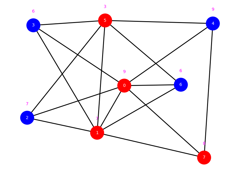
Let us first create an instance of the graph.

def create_graph(n, weighted):
    n = 8 # vertices
    weighted = True # Weighted or unweighted graph

    # Create graph through the networkx library
    g = nx.erdos_renyi_graph(n, 0.5)
    # Assign weights in the range {1, 2, ..., 10}, if the graph is weighted
    if weighted:
        weights = np.random.randint(1,10,size=n)
    else:
        weights = np.ones(n)

    # Adjacency matrix of g
    adj_matrix = nx.to_numpy_array(g)

    return g, adj_matrix, weights

def max_weight_sum_on_edges(weights, adj_matrix):
    weights = np.asarray(weights)
    
    # Get indices of the upper triangle where there is an edge
    # Computes the maximum w_i + w_j over all edges (i,j)
    i_indices, j_indices = np.triu_indices_from(adj_matrix, k=1)
    edge_mask = adj_matrix[i_indices, j_indices] > 0
    i_edges = i_indices[edge_mask]
    j_edges = j_indices[edge_mask]

    if len(i_edges) == 0:
        return 0  # No edges

    sum_weights = weights[i_edges] + weights[j_edges]
    return np.max(sum_weights)

n = 8
weighted = True
g, adj_matrix, weights = create_graph(n, weighted)
penalty_coeff = max_weight_sum_on_edges(weights, adj_matrix) + 1

node_size = 1000
# Display the graph
def display_graph(g, weighted):
    pos = nx.spring_layout(g, seed=42)
    nx.draw(
        g, pos,
        with_labels=True,
        node_color='blue',
        edge_color='black',
        node_size=node_size,
        font_color='white'
    )

    # Show vertices weights only if weighted
    if weighted:
        # Compute shifted positions (a bit higher than node centers)
        offset_pos = {k: (v[0], v[1] + 0.12) for k, v in pos.items()}
        weight_labels = {i: f"{w}" for i, w in enumerate(weights)}
        nx.draw_networkx_labels(
            g, offset_pos,
            labels=weight_labels,
            font_color='magenta',
            font_size=10
        )

    plt.show()

display_graph(g, weighted)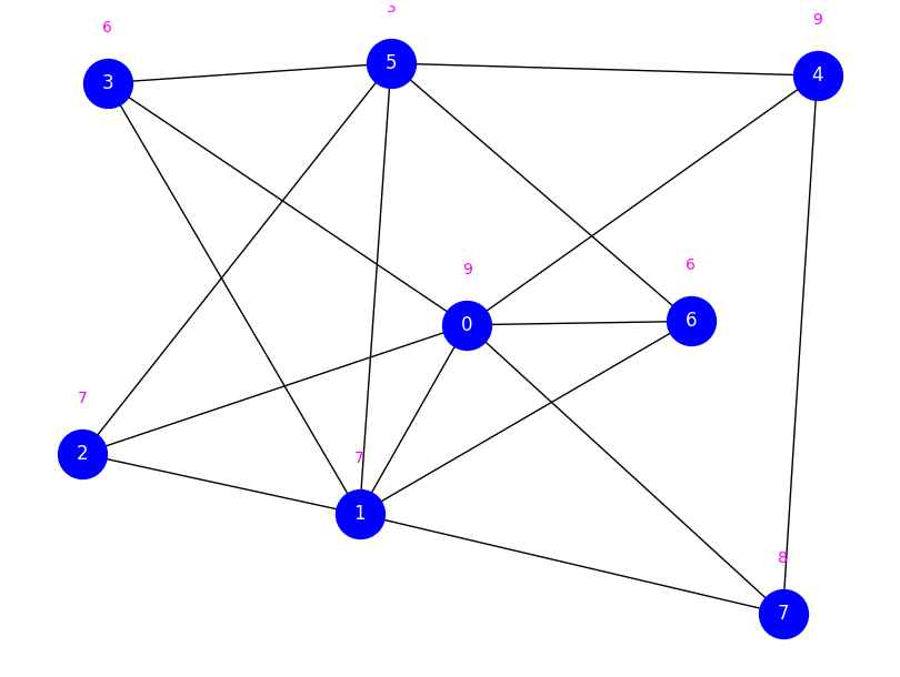

Brute forcing the solution space¶

@njit
def int_to_bitstring(i, n):
    # Converts an integer to its binary representation as a bitstring array of size n.
    if i > 0 and n < np.ceil(np.log2(i)):
        raise ValueError("Need larger n to encode the integer.")
    bits = np.empty(n, dtype=np.uint8)
    for j in range(n):
        bits[n - j - 1] = (i >> j) & 1
    return bits

@njit
def mis_cost(x, weights, adj_matrix, penalty_coeff):
    # Computes the MIS cost of a given vector x.
    w_term = 0.0
    penalty = 0.0
    n = x.shape[0]
    for i in range(n):
        if x[i] == 1:
            w_term += weights[i]
            for j in range(i + 1, n):
                if adj_matrix[i, j] and x[j] == 1:
                    penalty += 1
    return -w_term + penalty_coeff * penalty

# Compute cost for all bitstrings
def compute_all_costs(n,cost_fn,weights,adj_matrix,penalty_coeff):
    cost_values = []
    for i in range(2**n):
        bitstr = int_to_bitstring(i,n)         # convert integer to binary vector
        cost_val = cost_fn(bitstr,weights,adj_matrix,penalty_coeff)
        cost_values.append(cost_val)

    # Normalize to [0,1] (1 = minimum cost, 0 = maximum cost)
    cost_values = np.array(cost_values)
    min_val = cost_values.min()
    max_val = cost_values.max()
    normalized_values = 1 - (cost_values - min_val) / (max_val - min_val)

    # Create the dictionary: each key is a computational basis state (integer version) and the value is its quality (1 for optimal solutions, 0 for worst)
    return {i: normalized_values[i] for i in range(2**n)}

cost_quality_dict = compute_all_costs(n, mis_cost,weights,adj_matrix,penalty_coeff)

Let us now see the distribution of solution qualities, which are 1 for optimal solutions and 0 for worst.

plt.hist(cost_quality_dict.values(), bins=50, color='skyblue', edgecolor='black')
plt.xlabel('Cost Quality')
plt.ylabel('# of vectors')
plt.title('Histogram of the solution quality distribution')
plt.show()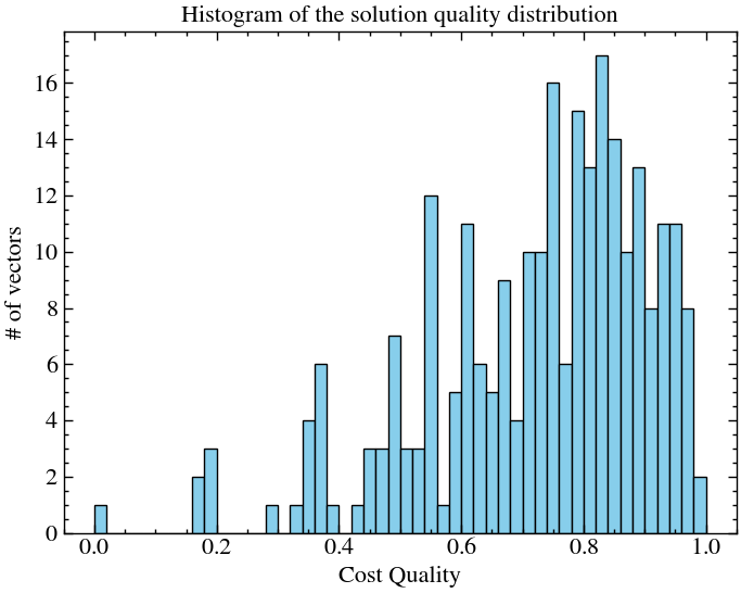

We can now visualize the cost function on the solution space ( $n$ -dimensional hypercube) where the color of the vertices depends on their quality.

# Solution graph (each node of this hypercube corresponds to a computational basis state, i.e. a decision)
mixer_graph = nx.hypercube_graph(n) # hypercube since we use X-mixer for this problem

# Map vertex -> value
node_colors = [cost_quality_dict[int("".join(map(str, node)), 2)] for node in mixer_graph.nodes()]

fig, ax = plt.subplots(figsize=(10, 6))
cmap = plt.cm.gist_rainbow

# Layout (spring or shell works well)
pos = nx.spring_layout(mixer_graph, seed=42)

# Draw graph
nodes = nx.draw_networkx_nodes(
    mixer_graph, pos, node_color=node_colors, cmap=cmap,
    vmin=0, vmax=1, node_size=50, ax=ax, alpha=0.7
)

nx.draw_networkx_edges(
    mixer_graph, pos,
    edge_color="gray",   # set all edges to gray
    alpha=0.5,
    ax=ax
)

# Add colorbar linked to nodes
cbar = fig.colorbar(nodes, ax=ax)
cbar.set_label("Quality")

ax.axis("off")
plt.show()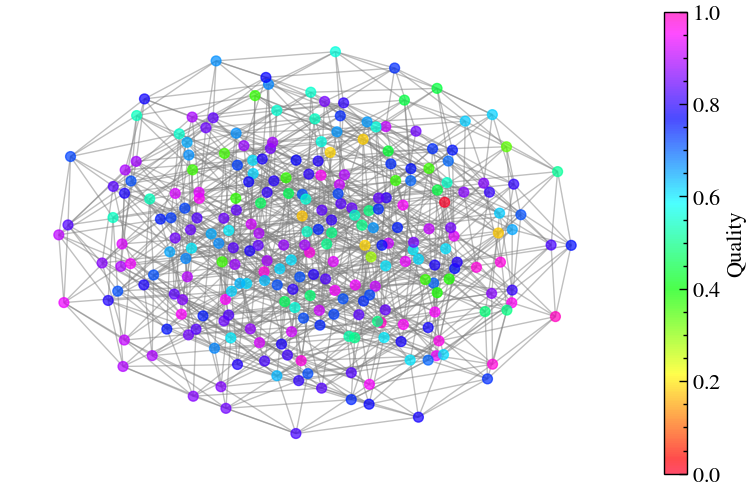

Step 2: The Sampling Walk Algorithm¶

Now, let us see the novel SamBa-GQW Sampling Walk algorithm, as the authors have provided here.

@njit
def bitstring_to_int(bits):
    # Converts a binary bitstring array to its integer representation.
    result = 0
    n = bits.size
    for j in range(n):
        result |= bits[n - j - 1] << j
    return result

def remove_duplicate_values(d):
    # Removes duplicate values in a dictionary based on hashable float representations.
    seen = set()
    result = {}
    for key, value in d.items():
        val = value.item() if hasattr(value, "item") else float(value)
        if val not in seen:
            seen.add(val)
            result[key] = val
    return result

@njit
def hamming_neighbors(bitvector):
    # Computes the neighbors of a hypercube vertex.
    neighbors = []
    n = bitvector.size
    for i in range(n):
        neighbor = bitvector.copy()
        neighbor[i] = 1 - neighbor[i]
        neighbors.append(bitstring_to_int(neighbor))
    return neighbors

class SamplingWalk:
    """
    SamplingWalk manages the initialization and manipulation of Hamiltonians
    for quantum sampling based on QAOA-like cost and mixer structure.

    Supports both QuTiP (NumPy, CPU): https://qutip.readthedocs.io/en/latest/index.html and dynamix
    """
    def __init__(self, n, cost, mixer, initial_state=None, use_density_matrix=False, local_mixer_gap=2,
                 use_qutip=True, convert_input_cost_fun=None,convert_input_neighbors_fun=None, cost_kwargs=None):
        """
        Parameters:
        - n: Size of the problem, i.e. number of binary variables.
        - cost: Array containing cost values of each solution or Function that computes the cost of a solution.
        - mixer: Array representing the connectivity of the mixer operator
        - initial_state: Quantum object of size 2^n representing the initial state of the system, if None it is set to uniform superposition
        - local_mixer_gap: Spectral gap of the local representation of the mixer
        - use_density_matrix: True if the states are to be represented with density matrices
        - use_qutip: True if the quantum simulation should be done with qutip, if False it is done with dynamiqs
        - convert_input_cost_fun: Function used to convert an integer to the correct input type of the cost function.
        - convert_input_neighbors_fun: Function used to convert an integer to the correct input type of the neighbors function 
        used in the sampling protocol.
        - cost_kwargs: Additional inputs of the cost function given as a dictionnary.
        """
        self.n_qubit = n
        self.mixer = mixer
        self.use_density_matrix = use_density_matrix
        self.local_mixer_gap = local_mixer_gap
        self.use_qutip = use_qutip
        self.initial_state = initial_state
        self.n_sample = 2 ** n
        self.sample = {}
        self.sampled_states = []
        self.collapse_op = []
        self.show_progress = False
        
        # Cost function input conversion
        if convert_input_cost_fun is None:
            self.convert_input_cost_fun = int_to_bitstring
        else:
            self.convert_input_cost_fun = convert_input_cost_fun
            
        # Cost function
        if callable(cost):
            self.cost_is_array = False
            base_cost = partial(cost, **cost_kwargs) if cost_kwargs else cost
            def wrapped_cost(x):
                if isinstance(x, numbers.Integral):
                    x = self.convert_input_cost_fun(x,self.n_qubit)
                return base_cost(x)
            self.cost = wrapped_cost
        else:
            self.cost = lambda x: cost[x]
            self.cost_is_array = True
            self.cost_array = cost
            
        # Neighbor function
        if convert_input_neighbors_fun is None:
            self.convert_input_neighbors_fun = int_to_bitstring
        else:
            self.convert_input_neighbors_fun = convert_input_neighbors_fun
        
        if use_qutip:
            import numpy as np
            self.np = np
            self.dtype = np.float64
        else:
            pass

        self.hopping = self.np.ones(2 ** n, dtype=self.dtype)
        self.t_list = self.np.linspace(0, 1, 2 ** n, dtype=self.dtype)

        self.qutip_initialization()

        self.first_energies = []
        self.first_mean_gaps = []
        self.energies = []
        self.mean_gaps = []
        self.dt = 1.
        self.gap_dt = 1
        
        # Hamiltonian evolution options
        self.store_states = True
        self.store_final_state = True
        self.n_steps = 10000
        
    def qutip_initialization(self):
        """
        Initialization of quantum objects with QuTip
        """
        from qutip import Qobj, basis, ket2dm, QobjEvo, sesolve, mesolve
        globals().update({"Qobj": Qobj, "basis": basis, "ket2dm": ket2dm, "QobjEvo": QobjEvo, "sesolve": sesolve, "mesolve": mesolve})

        if self.initial_state is None:
            vec = sum(basis(2 ** self.n_qubit, i) for i in range(2 ** self.n_qubit))
            self.initial_state = ket2dm(vec).unit() if self.use_density_matrix else vec.unit()
        else:
            self.initial_state = self.initial_state

        if not self.cost_is_array:
            cost_list = [self.cost(self.convert_input_cost_fun(x,self.n_qubit)) for x in range(2 ** self.n_qubit)]
            self.hc = Qobj(self.np.diag(self.np.array(cost_list, dtype=self.dtype)))
        else:
            self.hc = Qobj(self.np.diag(self.np.array(self.cost_array, dtype=self.dtype)))

        self.hd = Qobj(-self.mixer)
        self.hamiltonian = QobjEvo([[self.hd, self.hopping]], tlist=self.t_list) + self.hc

    def sample_without_conflicts(self, symmetry_fun=lambda x: []):
        """
        Samples `self.n_sample` unique integers from [0, 2**self.n_qubit) such that no sample violates
        constraints defined by symmetry_fun(bitstring). Efficient for large `self.n_qubit`.
    
        Parameters:
        - symmetry_fun: Function returning a list of conflicting integers for a sampled integer.
                        The input type of `symmetry_fun` must be that of `self.cost`
    
        Returns:
        - List of `self.n_sample` unique integers satisfying conflict constraints.
        """
        sampled_inputs: Set[str] = set()
        forbidden_inputs: Set[str] = set()
        sampled_integers: List[int] = []
    
        while len(sampled_integers) < self.n_sample:
            candidate = random.getrandbits(self.n_qubit)
            correct_cost_input = self.convert_input_cost_fun(candidate,self.n_qubit)
    
            if candidate in sampled_inputs or candidate in forbidden_inputs:
                continue
    
            conflicts = symmetry_fun(correct_cost_input)
            if any(conflict in sampled_inputs for conflict in conflicts):
                continue
    
            sampled_inputs.add(candidate)
            sampled_integers.append(candidate)
            forbidden_inputs.update(conflicts)
    
        return sampled_integers
    
    def sampling_protocol(self, q, neighbors_fun, symmetry_fun=lambda x: []):
        """
        Executes the sampling protocol.
        
        Parameters:
        - q: Number of sampled solutions.
        - neighbors_fun: Function that returns all the neighbors of a given solution.
                        The neighbors of a solution MUST be of type int.
        - symmetry_fun: Function that returns all the symmetric (known equivalent) of a given solution.
        """
        self.sampled_states = []
        self.n_sample = min(q, 2 ** self.n_qubit)
        energy = {}
        sample = self.sample_without_conflicts(symmetry_fun)
        min_gap_list = []
        min_gap_energy = []
        for guess in sample:
            guess_correct_cost_input = self.convert_input_cost_fun(guess,self.n_qubit)
            neighbors = neighbors_fun(self.convert_input_neighbors_fun(guess,self.n_qubit))
            gap_list = [self.cost(guess) - self.cost(ngb) for ngb in neighbors]
            positive_gap_list = [x for x in gap_list if x > 0]
            self.sampled_states.append(guess)
            if positive_gap_list:
                max_gap = max(positive_gap_list)
                min_gap = min(positive_gap_list)
                #min_gap_list.append(min(positive_gap_list))
                #min_gap_energy.append(guess)
                energy[guess] = (self.cost(guess), max_gap, min_gap)
                #energy[guess] = (self.cost(guess), max_gap)
        #energy[self.np.argmin(min(min_gap_list))] = (self.cost(self.np.argmin(min(min_gap_list))),min(min_gap_list))
        self.sample = energy

    def compute_mean_gaps(self):
        """
        Computes the mean gaps for each unique energy level.
        """
        energy_gap_dict = defaultdict(list)
        for val in self.sample.values():
            energy_gap_dict[float(val[0])].append(val[1])

        energy_mean = {
            e: self.np.mean(self.np.array(gaps, dtype=self.dtype)) / self.local_mixer_gap
            for e, gaps in energy_gap_dict.items()
        }
        energy_mean = remove_duplicate_values(energy_mean)
        sorted_energies = sorted(energy_mean.keys())
        sorted_mean_gaps = sorted([energy_mean[e] for e in sorted_energies])[::-1]

        self.energies = sorted_energies
        self.mean_gaps = sorted_mean_gaps
        self.first_energies = self.np.array(sorted_energies)
        self.first_mean_gaps = self.np.array(sorted_mean_gaps)

    def update_hamiltonian(self, t_list, hopping, hd, hc):
        """
        Updates the Hamiltonian.
    
        Parameters:
        - t_list: Array of time values.
        - hopping: Hopping rate function represented as an array.
        - hd: Mixer Hamiltonian.
        - hc: Cost Hamiltonian
        """
        self.t_list = t_list
        self.hopping = hopping
        self.hd = hd
        self.hc = hc
        
        if self.use_qutip:
            self.hamiltonian = QobjEvo([[hd, hopping]], tlist=t_list) + hc
        else:
            pass
        
    def interpolate(self, dt, gamma_list=[], annealing_time=True, t_max=1., stairs=False, cut=0., delta_min=0.,early_stop=0.,t_max_evolution=None):
        """
        Interpolates the hopping rate function.
    
        Parameters:
        - dt: Number of values for the interpolation.
        - gamma_list: Array containing the values gamma_k to be added to the hopping rate.
        - annealing_time: If True, the annealing time condition is respected.
        - t_max: Maximum time evolution, only counts if `annealing_time` is set to False.
        - stairs: True if the interpolation if piece-wise constant
        - cut: Minimum value allowed for the hopping rate
        - delta_min: Minimum gap difference allowed for the hopping rate
        """
        # If mean_gaps contains only one value, we must manually add values in the hopping rate for the interpolation
        if len(self.mean_gaps) == 1:
            raise ValueError("Not enough values to interpolate: add elements to gamma_list to solve this issue.")

        self.mean_gaps = self.first_mean_gaps[self.first_mean_gaps > cut]
        self.energies = self.first_energies[:len(self.mean_gaps)] 
        
        # We make sure that gamma_list is sorted in increasing order
        '''
        gamma_list = sorted(gamma_list)[::-1]
        
        gamma_list = [min(self.mean_gaps)] + gamma_list
        for i, gamma_k in enumerate(gamma_list[1:], 1):
            if gamma_k < gamma_list[i - 1] and gamma_k > cut:
                if self.use_qutip:
                    #self.mean_gaps.insert(-1,gamma_k) #self.mean_gaps.append(gamma_k)
                    #self.energies.insert(0, min(self.energies)-1)
                    self.mean_gaps = self.np.concatenate([self.mean_gaps,self.np.array([gamma_k])])
                    new_value = self.np.min(self.energies) - 1
                    self.energies = self.np.concatenate([self.np.array([new_value]), self.energies])
                else:
                    self.mean_gaps = self.np.concatenate([self.mean_gaps,self.np.array([gamma_k])])
                    new_value = self.np.min(self.energies) - 1
                    self.energies = self.np.concatenate([self.np.array([new_value]), self.energies])
        selected_gaps = [self.mean_gaps[0]]
        selected_energies = [self.energies[0]]
        for i in range(1,len(self.mean_gaps)):
            if self.np.abs(self.mean_gaps[i]-selected_gaps[-1]) >= delta_min:
                selected_gaps.append(self.mean_gaps[i])
                selected_energies.append(self.energies[i])

        if len(selected_gaps) > 1:
            self.mean_gaps = self.np.array(selected_gaps)
            self.energies = self.np.array(selected_energies)
        '''
        if annealing_time:
            annealing_time_list = []
            t = 0
            last_annealing_index = 0
            index_to_remove = []
            for i, gap in enumerate(self.mean_gaps):
                t_gap = self.np.pi / (2 * self.np.sqrt(2) * gap)
                if t_max_evolution is not None:
                    if t + t_gap <= t_max_evolution:
                        annealing_time_list.append(t+t_gap)
                        #print('Correct, gap:',gap,' Time:',t+t_gap,' tgap:',t_gap,' t:',t)
                        t += t_gap
                    elif t + gap <= t_max_evolution:
                        annealing_time_list.append(t+gap)
                        #print('Incorrect, gap:',gap,' Time:',t+gap)
                        t += gap
                    else:
                        index_to_remove.append(i)
                else:
                    annealing_time_list.append(t+t_gap)
                    t += t_gap
                '''
                if gap >= early_stop:
                    s += self.np.pi / (2 * self.np.sqrt(2) * gap)
                    annealing_time_list.append(s)
                    last_annealing_index = i
                else:
                    print('gap:',gap)
                    s += gap
                    annealing_time_list.append(s)
                '''

            if len(index_to_remove) > 0:
                self.mean_gaps = self.np.delete(self.mean_gaps,self.np.array(index_to_remove))
            #print(len(annealing_time_list),len(self.mean_gaps))
            #self.gap_dt = self.np.array(annealing_time_list)
            self.gap_dt = self.np.concatenate([self.np.array([0]),self.np.array(annealing_time_list)])
            '''
            if early_stop == 0:
                self.gap_dt = self.np.concatenate([self.np.array(annealing_time_list),self.np.array([s+annealing_time_list[last_annealing_index]])])
            else:
                self.gap_dt = self.np.concatenate([self.np.array(annealing_time_list),self.np.array([s+self.mean_gaps[-1]])])
            '''
            #self.gap_dt = self.np.concatenate([self.np.array(annealing_time_list),self.np.array([t+1e-2])])
            self.mean_gaps = self.np.concatenate([self.mean_gaps,self.np.array([0])])
            #print(len(self.gap_dt),len(self.mean_gaps))
        else:
            self.gap_dt = self.np.linspace(0, t_max, len(self.mean_gaps), dtype=self.dtype)
        
        if stairs:
            def stairs_interp(x, xp, fp):
                x = self.np.asarray(x,dtype=self.dtype)
                xp = self.np.asarray(xp,dtype=self.dtype)
                fp = self.np.asarray(fp,dtype=self.dtype)

                indices = self.np.searchsorted(xp, x, side='right') - 1
                indices = self.np.clip(indices, 0, len(fp) - 1)
                return self.np.take(fp, indices)

            # Define t_list as before
            t_list = self.np.linspace(self.gap_dt[0], self.gap_dt[-1], dt, dtype=self.dtype)

            # Compute hopping_interpolated using the stairs interpolation
            hopping_interpolated = stairs_interp(t_list, self.gap_dt, self.mean_gaps)
        else:
            interp_func = interp1d(self.gap_dt, self.mean_gaps, kind='linear', fill_value="extrapolate")
            t_list = self.np.linspace(self.gap_dt[0], self.gap_dt[-1], dt, dtype=self.dtype)
            hopping_interpolated = interp_func(t_list)

        self.dt = dt
        self.update_hamiltonian(t_list, self.np.array(hopping_interpolated), self.hd, self.hc)

    def evolve_qutip(self):
        """
        Hamiltonian evolution with QuTip.
        """
        options = {
            'store_states': self.store_states,
            'store_final_state': self.store_final_state,
            'nsteps': self.n_steps,
        }
        if self.show_progress:
            options['progress_bar'] = 'tqdm'
            
        if self.use_density_matrix:
            result = mesolve(self.hamiltonian, self.initial_state, self.t_list, self.collapse_op, e_ops=[self.hc], options=options)
        else:
            result = sesolve(self.hamiltonian, self.initial_state, self.t_list, e_ops=[self.hc], options=options)
        return result
        
    def evolve(self):
        """
        Hamiltonian evolution
        """
        return self.evolve_qutip()

    def settings(self,device='cpu',precision='single',show_progress=False):
        """
        Modifies the settings of QuTip/Dynamiqs.
    
        Parameters:
        - device: Device on which the evolution is computed, 'cpu', 'gpu' or 'tpu' (only for Dynamiqs).
        - precision: Floating point precision, 'single' (float32 & complex68) or 'double' (float64 & complex128) (only for Dynamiqs).
        - show_progress: If True, display the progress of the computation.
        """
        self.qutip_settings(show_progress)

    def qutip_settings(self,show_progress=False):
        """
        Modifies the settings of QuTip.
    
        Parameters:
        - show_progress: If True, display the progress of the computation.
        """
        self.show_progress = show_progress

mixer = nx.adjacency_matrix(nx.hypercube_graph(n)).todense() # dense representation: 2^n x 2^n matrix

samba_gqw = SamplingWalk(n,
            cost=mis_cost, # MIS cost function
            mixer=mixer, # Mixer (here n-dimensional hypercube)
            use_qutip=True, # QuTip or Dynamiqs
            use_density_matrix=False, # State vector representation
            convert_input_cost_fun=int_to_bitstring, # Function to convert integer to binary vectors
            cost_kwargs={'weights':weights, 'adj_matrix':adj_matrix, 'penalty_coeff':penalty_coeff} # Additional inputs of the cost function
        )

# Sampling protocol
q = n**2 # Quadratic sampling
neighbors_fun = hamming_neighbors # X-mixer (hypercube) neighboring function
samba_gqw.sampling_protocol(q=q, neighbors_fun=neighbors_fun) # sample n^2 vectors
samba_gqw.compute_mean_gaps()

We can visualize the vertices sampled on the solution graph.

# Map tuple nodes → integers
node_int_map = {node: int("".join(map(str, node)), 2) for node in mixer_graph.nodes()}

# Choose special nodes to highlight (integers from your sampler)
sampled_nodes = samba_gqw.sampled_states  # already integers

# Assign colors: red for special, skyblue otherwise
node_colors = [
    "red" if node_int_map[node] in sampled_nodes else "skyblue"
    for node in mixer_graph.nodes()
]

# Draw without labels
nx.draw(
    mixer_graph, pos,
    with_labels=False,
    node_color=node_colors,
    node_size=50,
    edge_color="gray", alpha=0.7
)
# Création de la légende
red_patch = mpatches.Patch(color='red', label='Sampled nodes')
blue_patch = mpatches.Patch(color='skyblue', label='Unsampled nodes')
plt.legend(handles=[red_patch, blue_patch])
plt.show()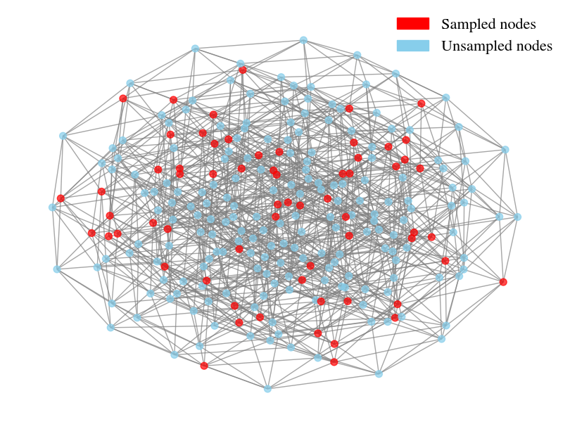

Interpolation of $\Gamma$ ¶

Now, let us construct the time-dependent hopping rate.

If we starts in a local superposition of states $\ket{j}$ and $\ket{k}$ , the probability of measuring the lower energy state $\ket{k}$ in this 2-state system is given by:

\begin{align*} \mathbb{P}_{jk}(t, \Gamma(E))=\frac{1}{2}+ \frac{\Gamma(E)\delta_{jk}}{\Gamma(E)^2 + \delta_{jk}^2}\sin\left(t\sqrt{\Gamma(E)^2 + \delta_{jk}^2}\right)^2, \end{align*}

(4)

where $\delta_{jk} = \Delta^C_{jk}/2$ . Under the balancing condition, $\Gamma^*_{jk} = \delta_{jk}$ . To find a good low energy solution, we maximise the probability, $\mathbb{P}_{jk}(t,\Gamma^*) = 1$ .

\begin{align*} \mathbb{P}_{jk}(t,\Gamma^*) = \frac{1}{2} + \frac{1}{2}&\sin\left(t\Gamma^*_{jk} \sqrt{2}\right)^2 = 1 \implies t^*_{jk} = \frac{\pi}{2\sqrt{2}\Gamma^*_{jk}}\\ \implies T^* &= \frac{\pi}{2\sqrt{2}}\sum_{jk \in E_M}\frac{1}{\Gamma^*_{jk}} \end{align*}

(5)

where $T*$ is the total evolution time to give the walker enough time to traverse all energy gaps, over the mixer edges $E_M$ .

In practice, we only have the approximate value of $\Gamma_{jk}$ , and we only have a poly( $n$ ) (in our case, $n^2$ ) number of sample edges $E_S$ instead of $E_M$ . So,

\begin{align*} T &= \frac{\pi}{2\sqrt{2}}\sum_{jk \in E_S}\frac{1}{\Gamma_{jk}} \end{align*}

(6)

which means that, our Hamiltonian evolution looks like,

\begin{align*} H(t_{jk}) = \Gamma\left(\frac{\pi}{2\sqrt{2}} t_{jk}\right)H_M+H_C \end{align*}

(7)

# Interpolation
samba_gqw.interpolate(dt=n**2)

# Create a figure with two subplots (1 row, 2 columns)
fig, axes = plt.subplots(1, 2, figsize=(14, 5))

# --- First plot ---
x_values = [val[0] for val in samba_gqw.sample.values()]
y_values = [val[1]/samba_gqw.local_mixer_gap for val in samba_gqw.sample.values()]

x_temp = samba_gqw.energies.copy()
new_temp = samba_gqw.np.concatenate([samba_gqw.np.array([samba_gqw.energies[0]]), x_temp])

axes[0].scatter(x_values, y_values, color='blue', label='Sampled energy gaps')
axes[0].scatter(samba_gqw.energies, samba_gqw.mean_gaps[::-1][1:], marker='s', facecolors='none', edgecolors='red', label="Sampled mean energy gaps")
axes[0].set_xlabel('Sampled cost value (energy)')
axes[0].set_ylabel('Energy gap')
axes[0].set_title('Sampled energies')
axes[0].legend()

# --- Second plot ---
# Scatter all points except last with hollow red squares
axes[1].scatter(samba_gqw.gap_dt[:-1], samba_gqw.mean_gaps[:-1], marker='s', facecolors='none', edgecolors='red', label='Sampled mean energy gaps')
# Scatter the last point in green (hollow)
axes[1].scatter(samba_gqw.gap_dt[-1:], samba_gqw.mean_gaps[-1:], marker='s', facecolors='none', edgecolors='lime', label='Zero energy point added')
# Plot interpolated hopping
axes[1].plot(samba_gqw.t_list, samba_gqw.hopping, color='blue', linestyle='-', linewidth=1.5, alpha=0.7, label="Interpolated hopping rate $\\Gamma(t)$")

axes[1].set_xlabel('$t$')
axes[1].set_ylabel('$\\Gamma$')
axes[1].set_title('Time-dependent hopping rate (annealing schedule)')
axes[1].legend()
plt.show()

Step 3: Hamiltonian Evolution¶

Now that the hopping schedule has been computed, we can finally run the quantum walk. In the continuous-time regime, this implies running $H$ for a time $T$ , as we calculated in the previous section (Method 1). In a gate-based quantum computer, this means that we need to discretize the evolution in time and implement a circuit (Method 2).

Method 1: Continuous Quantum Walk¶

# We perform the Hamiltonian evolution
results_cont = samba_gqw.evolve()

# We extract the results
results_array_cont = np.array([state.full() for state in results_cont.states]) # array of quantum states
times_cont = results_cont.times # values of evaluated time

Method 2: Quantum Circuit¶

To execute the continuous-time evolution on a gate-based quantum computer, the time-dependent Schrödinger equation must be discretized.

\begin{align*} i \hspace{0.7pt} \partial_t \ket{\psi(t)} = H(t) \ket{\psi(t)}; \text{ where } \ket{\psi(t)} = H(t)\ket{\psi(0)} \end{align*}

(8)

Using the Lie product formula, the corresponding unitary operator $U(t)$ is,

\begin{align*} U(t) = \lim_{p \to \infty} \left( \mathrm{e}^{-\frac{i}{p} \Lambda([0, t]) H_M } \mathrm{e}^{-\frac{i}{p} t H_C} \right)^p; \text{ where, } \Lambda([0, t]) = \int_0^{t} \Gamma(s) \mathrm{d}s \end{align*}

(9)

To maintain a manageable circuit depth while preserving accuracy, the evolution is split into nested time intervals: - Periods $\tau_l$ where the approximate hopping rate $\Gamma$ is linear. - Subintervals $p_l$ within those periods where Trotterization is applied.

Hence, for a given subinterval indexed by $r$ , the unitary $U(p,r)(T_l)$ is approximated as,

\begin{align*} U^{(p,r)}(T_l) &= \mathrm{e}^{-i\frac{\tau_l}{p_l} \Gamma_{l,r}H_M} \mathrm{e}^{-\frac{\tau_l}{p_l}H_C}\\ U(t) &= \prod_{l = 1}^{q}\left(\prod_{r = 1}^{p_l} U^{(p,r)}(T_l)\right) \end{align*}

(10)

Decomposing $U(t)$ into circuits¶

To decompose this circuit in terms of quantum gates, we split each

U^{(p, r)}(T_l) = U^{(p, r)}_M(T_l) U_C^{(p)}(T_l)

(11)

into

Mixer: $U_M^{(p, r)}(T_l)$ , The unitary implementation her for a hypercube (X-mixer) decomposes into rotation gates, because it is a sum of independent, single-qubit Pauli-X operators acting in parallel.

\begin{align*} U_M^{(p, r)}(T_l) &= \exp\left({-\frac{i \tau_l}{p_l} \Gamma_{l, r} H_M}\right),\\ U_M^{(p, r)}(T_l) &= \bigotimes_{b = 0}^{n-1} R^b_X \!\left( -2 \frac{\tau_l}{p_l} \Gamma_{l\!,r} \right). \end{align*}

(12)

Cost: The quantum circuit implementation of $U_C^{(p)}(T_l)$ consists of $\text{CNOT}$ and $R_Z$ for Quadratic/Higher order unconstrained binary optimization problems (Lucas et. al., 2014), and is dependent on the problem in question.

\begin{align*} U_C^{(p)}(T_l) &= \exp\left({- \frac{i \tau_l}{p_l} H_C}\right) \end{align*}

(13)

In particular, for the MIS problem, we can define the cost Hamiltonian from the MIS cost function as,

C(x)=-\sum_{i\in \mathcal{V}} w_ix_i+\lambda\sum_{(i,j)\in \mathcal{E}}x_ix_j.

(14)

Using the relation $x_i=(1-s_i)/2$ with $s_i\in\{-1,1\}$ , we rewrite the cost function with Ising variables:

\begin{aligned} C(s)&=-\frac{1}{2}\sum_{i\in \mathcal{V}}w_i+\frac{1}{2}\sum_{i\in \mathcal{V}}w_is_i+\frac{\lambda}{4}\sum_{(i,j)\in \mathcal{E}}(1-s_i-s_j+s_is_j) \\ &= \left(\frac{\lambda}{4}\lvert\mathcal{E} \rvert-\frac{1}{2}\sum_{i\in\mathcal{V}}w_i\right) + \frac{1}{2}\sum_{i\in\mathcal{V}}w_is_i -\frac{\lambda}{4}\sum_{(i,j)\in\mathcal{E}}(s_i+s_j) +\frac{\lambda}{4}\sum_{(i,j)\in\mathcal{E}}s_is_j. \end{aligned}

(15)

Constant term $\frac{\lambda}{4}\lvert\mathcal{E} \rvert-\frac{1}{2}\sum_{i\in\mathcal{V}}w_i$ is a global phase we can ignore, thus the cost Hamiltonian is:

H_C=\frac{1}{2}\sum_{i\in\mathcal{V}}w_i\sigma^Z_i -\frac{\lambda}{4}\sum_{(i,j)\in\mathcal{E}}\left(\sigma^Z_i+\sigma^Z_j\right)+\frac{\lambda}{4}\sum_{(i,j)\in\mathcal{E}}\sigma^Z_i\sigma^Z_j,

(16)

where $\sigma^Z_i$ is the Pauli- $Z$ matrix applied on qubit $i$ .

# MIS cost Hamiltonian
def cost_hamiltonian(n, cost_parameters, dt):
    qc = QuantumCircuit(n)
    q = qc.qubits

    g = cost_parameters[0]
    weights = cost_parameters[1]
    penalty_coeff = cost_parameters[2]

    for i in range(n):
        qc.rz(float(dt * weights[i]), q[i])

    # 2. Edge contributions
    for (j, k) in g.edges():
        qc.rz(-dt * penalty_coeff / 2.0, q[j])
        qc.rz(-dt * penalty_coeff / 2.0, q[k])

        qc.cx(q[j], q[k])
        qc.rz(dt * penalty_coeff / 2.0, q[k])
        qc.cx(q[j], q[k])

    return qc.to_gate(label='$H_C^{MIS}$')

# X-mixer Hamiltonian
def mixer_hamiltonian(n,gamma,dt):
    qc = QuantumCircuit(n)
    for i in range(n):
        qc.rx(-2.*gamma*dt, q[i])
    return qc.to_gate(label='$\\Gamma (t)H_M$')

# SamBa-GQW circuit
def sambaGQW_circuit(qc,samba_gqw,p,cost_hamiltonian,mixer_hamiltonian,cost_parameters,store_probabilities=False):
    n = samba_gqw.n_qubit
    
    # To store the probability vector after each layer of cost/mixer Hamiltonians for analysis purpose if store_probabilities=True
    probability_vector_list = []

    # Cost and mixer Hamiltonians
    for l in range(len(samba_gqw.mean_gaps)-1):
        for r in range(1,p[l]+1):
            tau_l = np.pi/(2*np.sqrt(2)*samba_gqw.mean_gaps[l])
            gamma_l_r = samba_gqw.mean_gaps[l] - (r+1/2)*((samba_gqw.mean_gaps[l]-samba_gqw.mean_gaps[l+1])/p[l])
            cost_hamiltonian_gate = cost_hamiltonian(n,cost_parameters,tau_l/p[l])
            mixer_hamiltonian_gate = mixer_hamiltonian(n,gamma_l_r,tau_l/p[l])

            qc.append(cost_hamiltonian_gate,qc.qubits)
            qc.append(mixer_hamiltonian_gate,qc.qubits)
            
            # Get the current probability vector after this step, we need to swap the qubits because of Qiskit ordering
            if store_probabilities:
                # Get the statevector probabilities
                prob = Statevector.from_instruction(qc).probabilities()
                # Reshape into n-dimensional tensor
                tensor = prob.reshape([2]*n)
                # Reverse qubit order
                tensor_reordered = tensor.transpose(list(reversed(range(n))))
                # Flatten back to vector
                prob_reordered = tensor_reordered.flatten()
                # Add it to the list
                probability_vector_list.append(prob_reordered)

    return qc, probability_vector_list

We construct the full quantum circuit that implements SamBa-GQW.

# List containing the number of subinterval per interval for hopping rate discretization (see Fig. 2 of the paper)
p = [5 for _ in range(len(samba_gqw.mean_gaps))] # here each interval is splitted into 5 subintervals

# We create our quantum circuit
q = QuantumRegister(n,name='q')
qc = QuantumCircuit(q)

# State preparation (uniform superposition for X-mixer)
qc.h(q)

# We create the circuit of SamBa-GQW (we can store probability vector at each layer, i.e. 1 unit of depth, for analysis purpose)
store_probabilities = True

# List containing the necessary objet needed to construct the cost Hamiltonian
cost_parameters = [g,weights,penalty_coeff]
qc, probability_vector_list = sambaGQW_circuit(qc,samba_gqw,p,cost_hamiltonian,mixer_hamiltonian,cost_parameters,store_probabilities=store_probabilities)

# Swaps for correct ordering (because of Qiskit ordering)
for i in range(n//2):
    qc.swap(q[i],q[n-i-1])

# Measurements in the computational basis
qc.measure_all()

# Draw the circuit
qc.decompose(reps=0).draw('mpl')

<Figure size 2252.61x16672.1 with 1 Axes>

# Number of measurements
n_shots = n**2

# We execute the circuit (results from the measurements)
sampler = SamplerV2()
job = sampler.run([qc.decompose(reps=1)], shots=n_shots)
job_result = job.result()
res_bitstr = job_result[0].data.meas.get_counts()
res = {}

# Map the values of res to probabilities
norm = np.sum(list(res_bitstr.values()))
for i in res_bitstr.keys():
    res[int(i,2)] = res_bitstr[i]/norm

# Get the correct probability vector (index i contains probability of measuring computational basis i)
prob_vector = np.zeros(2**n)

for idx, prob in res.items():
    prob_vector[idx] = prob

Step 4: Analyse the solutions¶

Now to assess the quality and correctness of our solutions, we define certain parameters, as follows.

Quality of a produced quantum state $\ket{\psi}$ is computed as,

\mathbf{q}(x)=\frac{C_{\max}-C(x)}{C_{\max}-C_{\min}}

We have already calculated this in step 2.

Distribution quality of a produced quantum state $\ket{\psi}$ is the expectation of its probability distribution,

\mathbb{E}[\psi] = \sum_{x\in\{0,1\}^n} \mathbf{p}(x)\cdot \mathbf{q}(x),

where $\mathbf{p}(x)= \lvert \braket{x|\psi} \rvert^2$ is the probability of measuring basis state $\ket{x}$ .

Participation ratio is used to quantify the localization of a state vector:

\text{PR}(\psi)=\left(2^n\sum_{x\in\{0,1\}}\mathbf{p}(x)^2\right)^{-1}

The uniform superposition leads to $\text{PR}=1$ and the fully localized state gives $\text{PR}=1/2^n$ . This metric gives information on the sparsity of $\ket{\psi}$ .

Ranking: labels the quality level of a decision $x$ . Optimal solutions have a ranking of 0, second-best decisions have a ranking of 1, and so on.

def rank_solutions_by_quality(quality_dict):
    """
    Parameters:
    - quality_dict: Dictionnary whose keys are integer representing quantum states and values are the associated quality.
    
    Returns:
    - Dictionnary whose keys are the rank and the values are list of integer representing the states.
    """
    quality_arr = np.array(list(quality_dict.values()))
    key_arr = np.array(list(quality_dict.keys()))

    # Get unique qualities and their inverse index mapping
    unique_qualities, inverse = np.unique(quality_arr, return_inverse=True)
    sorted_indices = np.argsort(-unique_qualities)  # descending

    # Map rank to list of keys
    rank_dict = {}
    for rank, q_idx in enumerate(sorted_indices):
        matching_keys = key_arr[inverse == q_idx].tolist()
        rank_dict[rank] = matching_keys

    return rank_dict

def distribution_quality(prob,quality):
    """
    Parameters:
    - prob: Array containing the probabilities of quantum states measurements.
    - quality: Array containing the quality of the solutions.
    
    Returns:
    - The quality of the distribution described by `prob`.
    """
    return np.dot(prob,quality)

Let us define a some performance/ranking plotting functions.

def plot_performance(distribution_quality_over_time,
                     participation_ratio_over_time,
                     probabilities_per_rank_over_time,
                     times,
                     quality_list,
                     rank_list,
                     rank_dict,
                     pourcentage=0,
                     error_type='sem',
                     distrib_error=None,
                     participation_error=None,
                     prob_per_rank_error=None,
                     save=False,
                     figname='perf.png',
                     marker_list=None,
                     markevery=1,
                     markersize=5,
                     show_colorbar=True,
                     show_legend=True,
                     fontsize_labels=12,
                     fontsize_data=10,
                     fontsize_legend=10,
                     legend_pos=(0,0),
                     xlabel='$t$'
):
    
    fig, ax = plt.subplots()
    
    # courbe distribution quality
    plt.plot(times, distribution_quality_over_time, 
             label='Distribution quality', color='orange', linestyle='--')
    if distrib_error is not None:
        plt.fill_between(times,
                         [m - e for m, e in zip(distribution_quality_over_time, distrib_error)],
                         [m + e for m, e in zip(distribution_quality_over_time, distrib_error)],
                         alpha=0.3, color='orange')
    
    # courbe participation ratio
    plt.plot(times, participation_ratio_over_time, 
             label='Participation ratio', color='lime', linestyle='dashdot')
    if participation_error is not None:
        plt.fill_between(times,
                         [m - e for m, e in zip(participation_ratio_over_time, participation_error)],
                         [m + e for m, e in zip(participation_ratio_over_time, participation_error)],
                         alpha=0.3, color='lime')
        
    if marker_list is None:
        marker_list = ["o","s","v","x","^","<",">","*","h","D","d","|","p",
           ".", ",", "1", "2", "3", "4", "8", "P", "H", "+", "X", "_"]

    total_ranks = len(probabilities_per_rank_over_time)
    all_ranks = set(range(total_ranks))
    individual_ranks = set(rank_list)
    other_ranks = list(all_ranks - individual_ranks)

    # Setup colormap
    # Setup colormap
    if show_colorbar:
        quality_array = np.array(quality_list)[rank_list]

        if np.min(quality_array) == np.max(quality_array):
            # Only one unique value: fix the range manually
            norm = colors.Normalize(vmin=0, vmax=1)
        else:
            norm = colors.Normalize(vmin=np.min(quality_array), vmax=np.max(quality_array))

        cmap = cm.cool
        sm = cm.ScalarMappable(cmap=cmap, norm=norm)
        sm.set_array([])

    
    # Plot individual ranks (sans labels pour la légende)
    for k, plot_rank_idx in enumerate(rank_list):
        mean_series = np.array(probabilities_per_rank_over_time[plot_rank_idx])
        err_series = (np.array(prob_per_rank_error[plot_rank_idx])
                      if prob_per_rank_error is not None else None)

        color = cmap(norm(quality_list[plot_rank_idx])) if show_colorbar else None

        line, = ax.plot(times, mean_series,
                        marker=marker_list[k],
                        markersize=markersize,
                        markerfacecolor='none',
                        markevery=markevery,
                        linestyle='-',
                        color=color,
                        alpha=1.)
        
        if err_series is not None:
            ax.fill_between(times,
                            mean_series - err_series,
                            mean_series + err_series,
                            alpha=0.2,
                            color=line.get_color())
    
    if other_ranks and pourcentage > 0:
        def top_percent(all_ranks, pourcentage):
            n = int(len(all_ranks) * pourcentage / 100)
            return all_ranks[:n]
        best_ranks = top_percent(list(rank_dict.keys()),pourcentage)
        #print(best_ranks)
        others_mean = np.sum([np.array(probabilities_per_rank_over_time[r]) for r in best_ranks], axis=0)

        ax.plot(times, others_mean,
                label="Probability "+str(pourcentage)+"\\% best rankings",
                linestyle='dotted',
                color='gray')

    # Axes
    ax.tick_params(axis='x', labelsize=fontsize_data)
    ax.tick_params(axis='y', labelsize=fontsize_data)
    ax.set_xlabel(xlabel, fontsize=fontsize_labels)

    # === Legend ===
    if show_legend:
        handles, labels = ax.get_legend_handles_labels()

        max_per_line = 4
        n_ranks = len(rank_list)

        # Split rank_list into chunks of size <= 4
        for chunk_start in range(0, n_ranks, max_per_line):
            chunk = rank_list[chunk_start:chunk_start + max_per_line]

            # Build the markers for this chunk
            combined_handles = tuple(
                Line2D([0], [0],
                       color=(cmap(norm(quality_list[r])) if show_colorbar else "black"),
                       linestyle="-",
                       marker=marker_list[i % len(marker_list)],
                       markerfacecolor="none",
                       markersize=markersize)
                for i, r in enumerate(chunk, start=chunk_start)
            )

            # Build the label string
            labels_str = ", ".join(str(r) for r in chunk)

            handles.append(combined_handles)
            labels.append(f"Probability rankings ({labels_str})")

        ax.legend(
            handles, labels,
            handler_map={tuple: HandlerTuple(ndivide=None)},
            loc="lower left",
            bbox_to_anchor=legend_pos,
            fontsize=fontsize_legend,
            frameon=True
        )
        plt.subplots_adjust(bottom=0.25)


    # Colorbar
    if show_colorbar:
        cbar = plt.colorbar(sm, ax=ax)
        cbar.set_label("Ranking quality", fontsize=fontsize_labels)
        cbar.ax.tick_params(labelsize=fontsize_data)

    plt.tight_layout()

    if save:
        plt.savefig(figname,dpi=300)

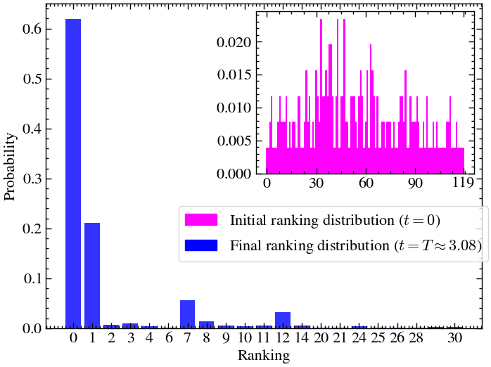
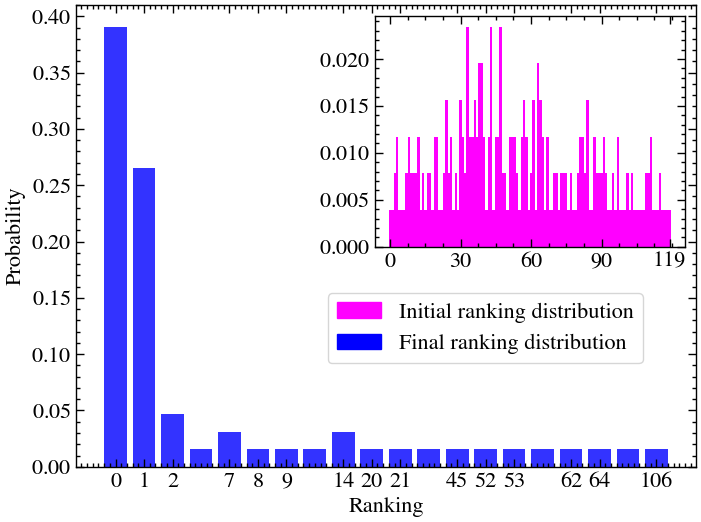
    plt.show()

def plot_ranking_distribution(prob_per_rank_final,
                              prob_per_rank_init=None,
                              threshold=1e-3,
                              num_ticks=15,
                              inset_plot_size=50,
                              inset_plot_label='Initial ranking distribution',
                              main_plot_label='Final ranking distribution',
                              save=False,
                              figname='ranking_distribution.png'
                              ):


    # Filter the data for the main plot
    filtered_indices = np.where(prob_per_rank_final > threshold)[0]
    filtered_values = prob_per_rank_final[filtered_indices]
    filtered_labels = filtered_indices
    filtered_x = np.arange(len(filtered_indices))

    # Create figure and main axis
    fig, ax = plt.subplots()
    bar_final = ax.bar(filtered_x, filtered_values, color='blue', alpha=0.8)
    ax.set_xlabel("Ranking")
    ax.set_ylabel("Probability")

    # Contrôle de la densité des ticks
    tick_indices = np.linspace(0, len(filtered_labels) - 1, num_ticks, dtype=int)
    tick_positions = filtered_x[tick_indices]
    tick_labels = [filtered_labels[i] for i in tick_indices]

    ax.set_xticks(tick_positions)
    ax.set_xticklabels(tick_labels)
    ax.tick_params(axis='x')

    # Inset axis
    if prob_per_rank_init is not None:
        ax_inset = inset_axes(ax, width=f"{inset_plot_size}%", height=f"{inset_plot_size}%", loc='upper right',bbox_to_anchor=(-0.00, 0.0005, 1, 1),  # (x0, y0, width, height)
            bbox_transform=ax.transAxes)
        x_inset = np.arange(len(prob_per_rank_init))
        bar_init = ax_inset.bar(x_inset, prob_per_rank_init, width=1., color='magenta', label='Initial ranking distribution', alpha=1)
        for bar in bar_init:
            bar.set_rasterized(True)
        # Compute 5 meaningful x-ticks
        size = len(x_inset)
        tick_positions = [0, size // 4, size // 2, 3 * size // 4, size - 1]
        tick_labels = [str(i) for i in tick_positions]

        ax_inset.set_xticks(tick_positions)
        ax_inset.set_xticklabels(tick_labels)
        ax_inset.tick_params(axis='y')
        ax.tick_params(axis='y')

    # Shared legend outside the plot (you can also put it inside with `loc=...`)
    final_patch = mpatches.Patch(color='blue', alpha=1, label=main_plot_label)
    init_patch = mpatches.Patch(color='magenta', alpha=1, label=inset_plot_label)

    if prob_per_rank_init is None:
        handles=[final_patch]
    else:
        handles=[init_patch, final_patch]
    ax.legend(handles=handles,
            loc='upper center',
            bbox_to_anchor=(0.66, 0.4),  # below the plot
            ncol=1, frameon=True)
    
    if save:
        plt.savefig(figname)

    plt.show()

For Method 1¶

Performance Metrics¶

Let us now see the performance metrics for solution obtained through both methods.

def plot_performace_and_ranking_ham(results_array, times):
    # We select the rankings for which we want to display the measurement probabilities over time
    rank_dict = rank_solutions_by_quality(cost_quality_dict)
    prob_over_time = [(np.abs(state)**2).reshape(-1) for state in results_array]
    distribution_quality_over_time = [distribution_quality(pr,list(cost_quality_dict.values())) for pr in prob_over_time]
    probabilities_per_rank_over_time = [[np.sum(pr[rank_dict[r]]) for pr in prob_over_time] for r in list(rank_dict.keys())]
    patricipation_ratio_over_time = 1 / (2**n * np.sum(np.vstack(prob_over_time)**2, axis=1))
    rank_to_display = [0,1,2,3]

    # We plot several metrics over time
    plot_performance(
        distribution_quality_over_time,
        patricipation_ratio_over_time,
        probabilities_per_rank_over_time,
        times,
        [cost_quality_dict[rank_dict[i][0]] for i in list(rank_dict.keys())],
        rank_list=rank_to_display,
        rank_dict=rank_dict,
        pourcentage=0,
        marker_list=None,
        markevery=20,
        markersize=6,
        show_colorbar=True,
        show_legend=True,
        save=False,
    )
    prob_per_rank_init = np.array([probabilities_per_rank_over_time[r][0] for r in list(rank_dict.keys())])
    prob_per_rank_final = np.array([probabilities_per_rank_over_time[r][-1] for r in list(rank_dict.keys())])

    plot_ranking_distribution(prob_per_rank_final=prob_per_rank_final,
        prob_per_rank_init=prob_per_rank_init,
        threshold=1e-3,
        num_ticks=20,
        inset_plot_size=50,
        inset_plot_label='Initial ranking distribution ($t=0$)',
        main_plot_label=f'Final ranking distribution ($t=T\\approx {times[-1]:.2f}$)',
        save=False,)
    
    return prob_over_time, rank_dict, prob_per_rank_init

prob_over_time, rank_dict, prob_per_rank_init = plot_performace_and_ranking_ham(results_array_cont, times_cont)

Conduct Measurement¶

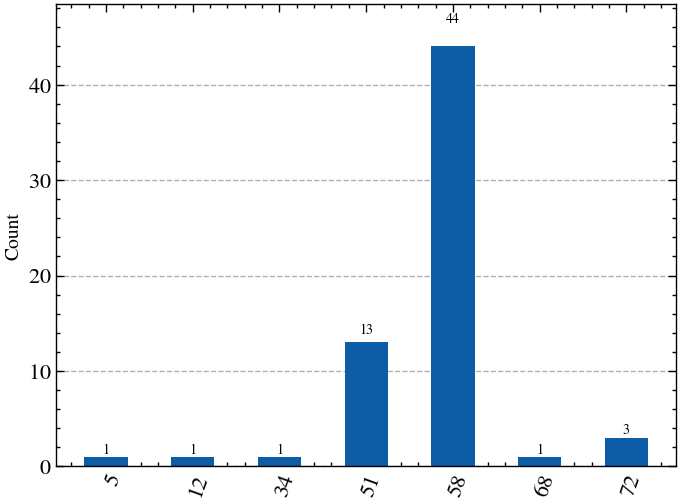
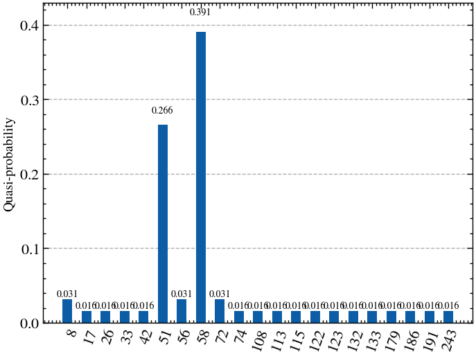
We simulate measurements in the computational basis and we select the best found approximation to be the measured state with lowest cost.

def sample_measurements(probabilities, k, seed=None):
    """
    Simulate k measurements from a probability distribution.
    
    Args:
        probabilities (array-like): probability vector that sums to 1
        k (int): number of measurements
        seed (int, optional): random seed for reproducibility
    
    Returns:
        dict: {index: count of times measured}
    """
    rng = np.random.default_rng(seed)
    n = len(probabilities)
    outcomes = rng.choice(np.arange(n), size=k, p=probabilities)
    counts = dict(Counter(outcomes))
    return counts

# Number of measurements
n_shots = n**2

# Simulate the measurements
res = sample_measurements(prob_over_time[-1], n_shots, seed=42)

# Print the best found assignment
best_found_assigment = min(res.keys(), key=lambda b: mis_cost(int_to_bitstring(b,n),weights,adj_matrix,penalty_coeff))
print(f"The best found assignment is x={best_found_assigment} "
      f"({format(best_found_assigment, f'0{n}b')}) "
      f"of ranking r={next((key for key, values in rank_dict.items() if best_found_assigment in values))}")

# Plot the results of the measurements
plot_histogram(res)

The best found assignment is x=58 (00111010) of ranking r=0

def plot_best_solution(best_found_assigment):
    # Plot the best found assignment
    node_colors = ['blue' if int_to_bitstring(best_found_assigment,n)[i] else 'red' for i in range(n)]

    pos = nx.spring_layout(g, seed=42)
    nx.draw_networkx_nodes(g, pos, node_color=node_colors, node_size=node_size)
    nx.draw_networkx_edges(g, pos, width=2, alpha=1, edge_color="black", style="solid")

    # Display node labels (indices)
    nx.draw_networkx_labels(g, pos, font_size=10, font_color="white")

    # Edge labels if weighted
    if weighted:
        # Compute shifted positions (a bit higher than node centers)
        offset_pos = {k: (v[0], v[1] + 0.12) for k, v in pos.items()}
        weight_labels = {i: f"{w}" for i, w in enumerate(weights)}
        nx.draw_networkx_labels(
            g, offset_pos,
            labels=weight_labels,
            font_color='magenta',
            font_size=10
        )

    ax = plt.gca()
    ax.margins(0.08)
    plt.axis("off")
    plt.tight_layout()
    print(f"Displayed assignment: x={best_found_assigment} ({format(best_found_assigment, f'0{n}b')})")
    plt.show()

plot_best_solution(best_found_assigment)

Displayed assignment: x=58 (00111010)

For Method 2¶

Performance Metrics¶

# Number of measurements
n_shots = n**2

# We execute the circuit (results from the measurements)
sampler = SamplerV2()
job = sampler.run([qc.decompose(reps=1)], shots=n_shots)
job_result = job.result()
res_bitstr = job_result[0].data.meas.get_counts()
res = {}

# Map the values of res to probabilities
norm = np.sum(list(res_bitstr.values()))
for i in res_bitstr.keys():
    res[int(i,2)] = res_bitstr[i]/norm

# Get the correct probability vector (index i contains probability of measuring computational basis i)
prob_vector = np.zeros(2**n)

for idx, prob in res.items():
    prob_vector[idx] = prob

We compute again several metrics over time for analysis purposes and plot them (only if we store probabilities during the circuit).

if store_probabilities:
    # Metrics
    prob_over_time_circuit = probability_vector_list
    distribution_quality_over_time_circuit = [distribution_quality(pr,list(cost_quality_dict.values())) for pr in prob_over_time_circuit]
    probabilities_per_rank_over_time_circuit = [[np.sum(pr[rank_dict[r]]) for pr in prob_over_time_circuit] for r in list(rank_dict.keys())]
    patricipation_ratio_over_time_circuit = 1 / (2**n * np.sum(np.vstack(prob_over_time_circuit)**2, axis=1))

    # We select the rankings for which we want to display the measurement probabilities over time
    rank_to_display = [0,1,2,3]

    # We plot several metrics over time
    plot_performance(
        distribution_quality_over_time_circuit,
        patricipation_ratio_over_time_circuit,
        probabilities_per_rank_over_time_circuit,
        np.arange(1,len(prob_over_time_circuit)+1),
        [cost_quality_dict[rank_dict[i][0]] for i in list(rank_dict.keys())],
        rank_list=rank_to_display,
        rank_dict=rank_dict,
        pourcentage=0,
        save=False,
        figname='mis.png',
        marker_list=None,
        markevery=20,
        markersize=6,
        show_colorbar=True,
        show_legend=True,
        xlabel='Depth (number of cost and mixer layers)'
    )

probabilities_per_rank_measurements = [np.sum(prob_vector[rank_dict[r]]) for r in list(rank_dict.keys())]
prob_per_rank_final_circuit = np.array([probabilities_per_rank_measurements[r] for r in list(rank_dict.keys())])

plot_ranking_distribution(prob_per_rank_final=prob_per_rank_final_circuit,
        prob_per_rank_init=prob_per_rank_init, # computed in the Hamiltonian evolution part
        threshold=1e-3,
        num_ticks=15,
        inset_plot_size=50,
        inset_plot_label='Initial ranking distribution',
        main_plot_label='Final ranking distribution',
        save=False,)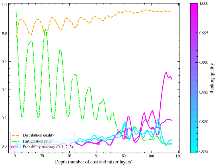

Conduct Measurement¶

We select the measured computational state with the lowest cost to be our best approximation.

# Print the best found assignment
best_found_assigment = min(res.keys(), key=lambda b: mis_cost(int_to_bitstring(b,n),weights,adj_matrix,penalty_coeff))
print(f"The best found assignment is x={best_found_assigment} "
      f"({format(best_found_assigment, f'0{n}b')}) "
      f"of ranking r={next((key for key, values in rank_dict.items() if best_found_assigment in values))}")

# Plot the results of the measurements
plot_histogram(res)

The best found assignment is x=58 (00111010) of ranking r=0

plot_best_solution(best_found_assigment)

Displayed assignment: x=58 (00111010)

Linear vs. Quadratic vs. Cubic Sampling¶

Let us see the difference between three sampling methods for a graph with 10 vertices.

n = 10
weighted = True
g, adj_matrix, weights = create_graph(n, weighted)
penalty_coeff = max_weight_sum_on_edges(weights, adj_matrix) + 1
display_graph(g, weighted)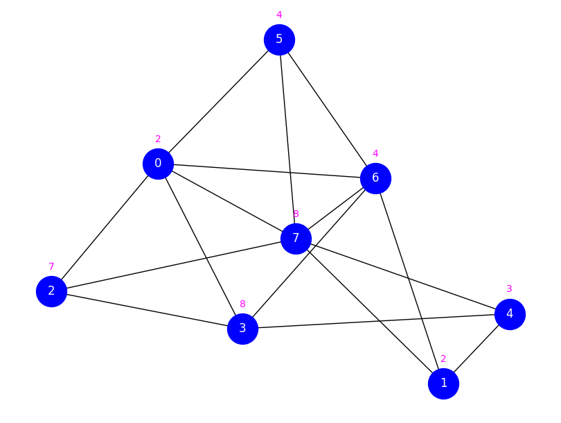

cost_quality_dict = compute_all_costs(n, mis_cost,weights,adj_matrix,penalty_coeff)
mixer = nx.adjacency_matrix(nx.hypercube_graph(n)).todense() # dense representation: 2^n x 2^n matrix

samba_gqw = SamplingWalk(n,
            cost=mis_cost, # MIS cost function
            mixer=mixer, # Mixer (here n-dimensional hypercube)
            use_qutip=True, # QuTip or Dynamiqs
            use_density_matrix=False, # State vector representation
            convert_input_cost_fun=int_to_bitstring, # Function to convert integer to binary vectors
            cost_kwargs={'weights':weights, 'adj_matrix':adj_matrix, 'penalty_coeff':penalty_coeff} # Additional inputs of the cost function
        )

def run_samba_gqw_with_sampling(q):
    neighbors_fun = hamming_neighbors # X-mixer (hypercube) neighboring function
    samba_gqw.sampling_protocol(q=q, neighbors_fun=neighbors_fun) # sample n^2 vectors
    samba_gqw.compute_mean_gaps()
    # Interpolation
    samba_gqw.interpolate(dt=q)
    # We perform the Hamiltonian evolution
    results1 = samba_gqw.evolve()
    results_array1 = np.array([state.full() for state in results1.states]) # array of quantum states
    times1 = results1.times 

    rank_dict = rank_solutions_by_quality(cost_quality_dict)
    prob_over_time = [(np.abs(state)**2).reshape(-1) for state in results_array1]
    distribution_quality_over_time = [distribution_quality(pr,list(cost_quality_dict.values())) for pr in prob_over_time]
    probabilities_per_rank_over_time = [[np.sum(pr[rank_dict[r]]) for pr in prob_over_time] for r in list(rank_dict.keys())]
    patricipation_ratio_over_time = 1 / (2**n * np.sum(np.vstack(prob_over_time)**2, axis=1))
    rank_to_display = [0,1,2,3]

    # We plot several metrics over time
    plot_performance(
        distribution_quality_over_time,
        patricipation_ratio_over_time,
        probabilities_per_rank_over_time,
        times1,
        [cost_quality_dict[rank_dict[i][0]] for i in list(rank_dict.keys())],
        rank_list=rank_to_display,
        rank_dict=rank_dict,
        pourcentage=5,
        marker_list=None,
        markevery=20,
        markersize=6,
        show_colorbar=True,
        show_legend=True,
        save=False,
    )

run_samba_gqw_with_sampling(n**1)
run_samba_gqw_with_sampling(n**2)
run_samba_gqw_with_sampling(n**3)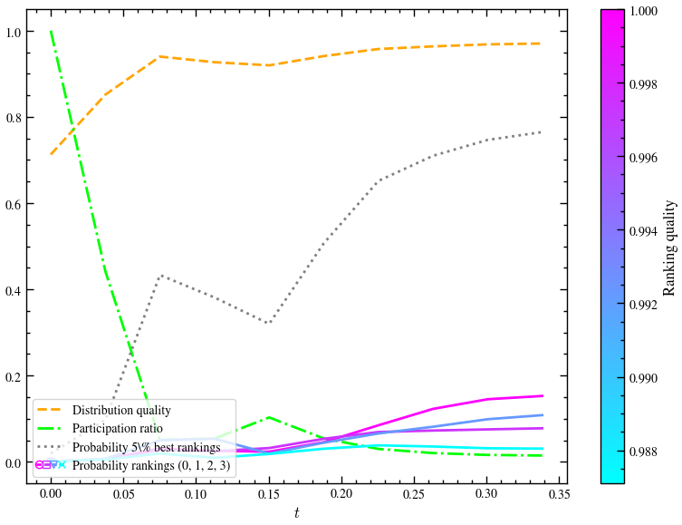

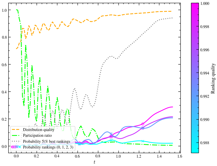
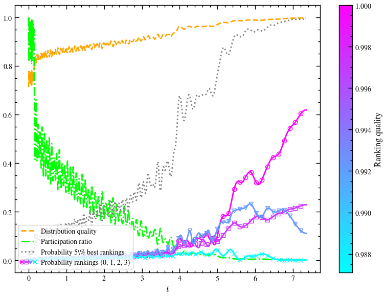
Key Takeaways¶

From the above three graphs, consider the probability of the 5% best rankings and how it changes for sampling $n$ , $n^2$ and $n^3$ respectively. Even with $n=10$ , we see that after a certain time $t$ , the probability approaches 1. There is a significant jump of this probability from $n$ to $n^2$ . However, the jump from $n^2$ to $n^3$ is relatively lower.

As the exponent of $n$ increases, naturally, we will get better and better results. We have seen the $n=10$ case here. The paper claims $n=20$ , the change between $n^2$ and $n^3$ is basically negligible, meaning that for such problems, we can get away quadratic sampling.

$\therefore$ Quadratic sampling is good enough, especially for large enough $n$ ( $\ge 10$ ).

Scaling¶

Let us see the runtmie scaling of this algorithm in $n$ , and also compare it to the classical method.

import time
import itertools

# Find independent set using brute force method
def is_independent_set(subset, adjacency_matrix):
    for i in range(len(subset)):
        for j in range(i + 1, len(subset)):
            u, v = subset[i], subset[j]
            # If an edge exists, it's not an independent set
            if adjacency_matrix[u][v] == 1:
                return False
    return True

def find_maximum_independent_set(adjacency_matrix):
    n = len(adjacency_matrix)
    vertices = list(range(n))
    
    # Check subsets starting from the largest possible size
    for size in range(n, 0, -1):
        for subset in itertools.combinations(vertices, size):
            if is_independent_set(subset, adjacency_matrix):
                return list(subset) # Return the first (largest) one found
    
    return []

def compute_runtime(n):
        weighted = True
        g, adj_matrix, weights = create_graph(n, weighted)
        penalty_coeff = max_weight_sum_on_edges(weights, adj_matrix) + 1
        cost_quality_dict = compute_all_costs(n, mis_cost,weights,adj_matrix,penalty_coeff)
        mixer = nx.adjacency_matrix(nx.hypercube_graph(n)).todense() # dense representation: 2^n x 2^n matrix
        samba_gqw = SamplingWalk(n,
                cost=mis_cost, # MIS cost function
                mixer=mixer, # Mixer (here n-dimensional hypercube)
                use_qutip=True, # QuTip or Dynamiqs
                use_density_matrix=False, # State vector representation
                convert_input_cost_fun=int_to_bitstring, # Function to convert integer to binary vectors
                cost_kwargs={'weights':weights, 'adj_matrix':adj_matrix, 'penalty_coeff':penalty_coeff} # Additional inputs of the cost function
                )
        q = n**2
        neighbors_fun = hamming_neighbors # X-mixer (hypercube) neighboring function
        samba_gqw.sampling_protocol(q=q, neighbors_fun=neighbors_fun) # sample n^2 vectors
        samba_gqw.compute_mean_gaps()
        # Interpolation
        samba_gqw.interpolate(dt=q)
        # We perform the Hamiltonian evolution

        start1 = time.perf_counter()
        results1 = samba_gqw.evolve()
        end1 = time.perf_counter()

        start2 = time.perf_counter()
        mis = find_maximum_independent_set(adj_matrix)
        end2 = time.perf_counter()

        return end1 - start1, end2 - start2

runtimes_h = []
runtimes_b = []
for i in range(3, 11):
    r1, r2 = compute_runtime(i)
    runtimes_h.append(r1)
    runtimes_b.append(r2)

qs = [3, 4, 5, 6, 7, 8, 9, 10]
plt.plot(qs, runtimes_h/np.max(runtimes_h), label='Hamiltonian Evolution')
plt.plot(qs, runtimes_b/np.max(runtimes_b), label='Brute Force')
plt.xlabel('# of vertices')
plt.ylabel('Time taken to Run')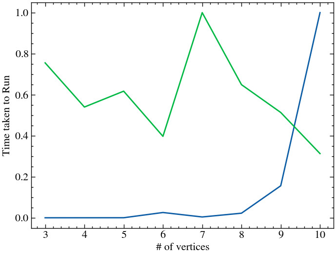

In case of the classical algorihm, for values of $n$ as small as 10, the total number of possible solutions is $2^10=1024$ , which is still quite small for a standard computer, hence we see no scaling. To see any real effects, we need to go see the behavious as $n\rightarrow \infty$ . We can also see that unfortunately, SamBa-GQW still scales exponentially with time. Since we are running the algorithm on a classical computer, this makes sense, since the time taken for qikskit to work with $n$ quibits will also essentially scale exponentially. To see any noticable effects, we need to run the algorithm on a quantum computer. For the purposes of this project, I was not able to successfully run it on cloud platform in time, despite repeated efforts.

Conclusions¶

We have seen that the SamBa-GQW algorithm successfully shifts an initial uniform distribution into a very localized distribution around the optimal solution in a short evolution time.
For problems up to size $n = 20$ , sampling just $n^2$ states empirically yields high-quality approximate solutions.
SamBa-GQW outperforms the original variational GQW by reducing classical execution time by at least one order of magnitude (e.g., from 24 hours to 9 minutes on n = 20, as seen in the original paper)
By completely bypassing the need for a classical optimizer, it guarantees more stable scaling and avoids the common pitfalls of GQWs (like exponenial scaling and parameter dependency).

Future Possibilities¶

The authors could have performed more rigorous testing by testing the algorithm on a quantum computer and measure how it really scales with $n$ .
They could also have done more to explore the asymptotic scaling of the “offline classical sampling protocol”. They could have detailed how the samples required for qubits behave as it grows, particularly for instances beyond 20 qubits. One could possibly constraint the maximum power of $n$ needed for the sampling to be safe enough to use.
While they tested several quadratic and polynomial problems, they could have applied the methodology to a wider array of NP-hard combinatorial optimization problems with complex constraints (e.g., job scheduling or large TSP instances) to test the robustness of the guiding protocol.
The authors could have investigated, for example, the optimal ways to structure the time-dependent hopping rate beyond the proposed approach, perhaps exploring different types of graph structures for the quantum walk

References¶

Nzongani, U., Mermoud, D. L., Di Molfetta, G., & Simonetto, A. (2025). Sampled-Based Guided Quantum Walk. arXiv. 10.48550/ARXIV.2509.15138
Albash, T., & Lidar, D. A. (2018). Adiabatic quantum computation. Reviews of Modern Physics, 90(1). 10.1103/revmodphys.90.015002
Schulz, S., Willsch, D., & Michielsen, K. (2024). Guided quantum walk. Physical Review Research, 6(1). 10.1103/physrevresearch.6.013312
Lucas, A. (2014). Ising formulations of many NP problems. Frontiers in Physics, 2. 10.3389/fphy.2014.00005

Introduction¶

Formulating the problem¶

Quantum Walk Implementation¶

Guided Quantum Walk¶

Aim of the Paper¶

Maxmimum Independent Set Problem: SamBa-GQW Step-by-Step¶

Step 1: Initialise the problem¶

Brute forcing the solution space¶

Step 2: The Sampling Walk Algorithm¶

Interpolation of Γ\GammaΓ¶

Step 3: Hamiltonian Evolution¶

Method 1: Continuous Quantum Walk¶

Method 2: Quantum Circuit¶

Decomposing U(t)U(t)U(t) into circuits¶

Step 4: Analyse the solutions¶

For Method 1¶

Performance Metrics¶

Conduct Measurement¶

For Method 2¶

Performance Metrics¶

Conduct Measurement¶

Linear vs. Quadratic vs. Cubic Sampling¶

Key Takeaways¶

Scaling¶

Conclusions¶

Future Possibilities¶

Interpolation of $\Gamma$ ¶

Decomposing $U(t)$ into circuits¶