Markovian Agent Based Monte Carlo Simulations - Computational Physics Projects

for Reaction-Diffusion Models, Population Dynamics, and Epidemic Spreading

Introduction¶

In agent-based Monte Carlo simulations, we implement the microscopic stochastic reaction processes as a Markov chains -- which basically mean that the updated configurations depend only on the immediately past states, and transitions between them depend on probabilities that we can control.

Aim of the Paper¶

The goal of performing Monte-Carlo Simulations is not to fully reflect a system’s behavior on all scales, but to capture its qualitative features at sufficiently long times and distances, including temporal oscillations or spatial structures. In the paper, the authors use simulations of reaction–diffusion systems, stochastic models for population dynamics (i.e. the Lotka-Volterra model) and epidemic spreading, to highlight some of the interdisciplinary aspects of such computational methods, while also adressing potential pitfalls, error sources and data analysis methods to properly quantify certain qualitative features which can only be achieved stochastically.

Step-by-Step Simulation Setup¶

We first need to establish the rules of the world.

Agents: Indistinguishable passive (or active) particles belonging to a species that are subject to certain reactive processes.
Simulation space: Particles are allowed to move or hop between sites on a lattice -- lattice sites may be constrained by a finite carrying capacity.
Reactive process: Particles may interact with themselves or with other particles of their own species or another species.

Now, once the initial setup is completed, we run the simulation.

At each step, one particle is randomly selected from the space and subjected to reactive processes based on predefined probabilities.
Time evolution: A Monte Carlo step (MCS) is complete when each particle that was present at the start of the step was selected once on average.
Observables: We use Master equations to track observables as the simulation evolves.

Alert: Make sure all necessary python packages are installed.

!pip install scienceplots
!pip install numba-progress

import numpy as np
from matplotlib.colors import ListedColormap
from numba import njit, prange, objmode#, vectorize, types
import matplotlib.pyplot as plt
import scienceplots
plt.style.use(['science', 'notebook', 'no-latex'])
from matplotlib import animation
from IPython.display import HTML
import time
from scipy.integrate import solve_ivp
from numba_progress import ProgressBar

@njit
def random_pick(array):
    return array[int(np.random.random()*len(array))]

@njit
def bincount(data, num_bins):
    counts = np.zeros(num_bins+1, dtype=np.int32)
    for val in data:
        counts[val] += 1
    return counts

@njit
def weighted_choice(items, probabilities):
    # Numba-compatible replacement for rng.choice(items, p=probabilities)
    r = np.random.random()
    cumulative_p = 0.0
    for i in range(len(probabilities)):
        cumulative_p += probabilities[i]
        if r < cumulative_p:
            return items[i]
    return items[0] # Fallback for rounding issues

Reaction-Diffusion Modelling¶

We will first consider the simplest forms of reaction-diffusion models. First let us define a general function to perform monte-carlo simulations of one-dimensional annihilation reactions.

# @njit("Tuple([float64[:,:], f8[:,:], f8[:,:]])(i8,i8,i8,i8[:],float64,float64)",)
@njit
def run_coagulation(perform_world_rules, ntimes, L, T, species_list, initialise_randomly=True, *args):
    nspecies = len(species_list)
    number_density_average = np.zeros((ntimes, T, nspecies))
    hops_per_step_average = np.zeros((ntimes, T-1))

    # run the simulation ntimes number of times
    for itime in prange(ntimes):

        world_evolution = np.zeros((T, L), dtype=np.int32) # world as it evolves
        if initialise_randomly:
            world = np.array([int(np.random.random()*nspecies) for _ in range(L)]) # start with all sites filled randomly
        else:
            world = np.array([x%nspecies for x in range(L)]) # start with all sites occupied uniformly

        world_evolution[0] = world
        hops_per_step = np.zeros(T-1)
        number_density_average[itime, 0] = bincount(world, nspecies)[:-1]

        for ti in range(1, T):
            world = world_evolution[ti-1] # previous iteration

            # current occupant density = number of +ve entries
            N = L - bincount(world, nspecies)[-1]
            hops_this_step = 0
            
            # one monte carlo step
            for nj in range(N): 
                possible_locs = np.where(world > -1)[0]
                loc = random_pick(possible_locs)
                loc = -1 if loc == L-1 else loc # periodic boundary condition
                
                world, hops = perform_world_rules(world, loc, *args)
                hops_this_step += hops

            world_evolution[ti] = world
            number_density_average[itime, ti] = bincount(world, nspecies)[:-1]
            hops_per_step[ti-1] = hops_this_step/N if N !=0 else 0

        hops_per_step_average[itime, :] = hops_per_step

    # return the last world_evolution array (only for visualisation purposes)
    return world_evolution, number_density_average, hops_per_step_average

Single Species Annihilation¶

They are equations of the form,

2A \rightarrow A

(1)

Basically, once we define a world populated with A particles, if two A particles come into contact with each other, they essentially coagulate, which means that one engulfs the other. We can implement this in python using the following code.

@njit
def single_species_coagulation(world, loc, *params):
    hopping_rate = params[0]
    coagulation_rate = params[1]
    hops = 0
    if np.random.random() < hopping_rate: # hop or not
        possible_hops = []
        if world[loc-1] == -1:
            possible_hops.append(-1)
        if world[loc+1] == -1:
            possible_hops.append(+1)
        
        if possible_hops:
            hops +=1 
            chosen_hop = possible_hops[int(np.random.random()*len(possible_hops))]
            world[loc + chosen_hop], world[loc] = 0, -1

    # coagulation
    if np.random.random() < coagulation_rate: # coagulate or not
        possible_coagulates = []
        if world[loc-1] == 0:
            possible_coagulates.append(-1)
        if world[loc+1] == 0:
            possible_coagulates.append(+1)

        if possible_coagulates:
            # hops += 1
            chosen_target = possible_coagulates[int(np.random.random()*len(possible_coagulates))]
            world[loc + chosen_target] = -1
    return world, hops

L, T = 300, 200
hopping_rate = 0.3
coagulation_rate = 0.05
ntimes = 300
world_evolution_last, number_densities, hops_per_step = run_coagulation(single_species_coagulation, ntimes, L, T, [0], True, hopping_rate, coagulation_rate)

xi = np.arange(0,L)
yi = np.arange(0,T)
xi, yi = np.meshgrid(xi, yi)

plt.figure(figsize=(12, 6))
cmap = ListedColormap(['k', 'r'])
plt.imshow(world_evolution_last, cmap=cmap, origin='lower')
plt.xlabel('$x$')
plt.ylabel('Time')
plt.gca().invert_yaxis()
plt.minorticks_on()
plt.title('Visualizing the Last Monte Carlo Run\n$\\langle n_A(0) \\rangle = 1, r_\\text{hopping}$ = ' + str(hopping_rate) + ', $r_\\text{coagulation}=$' + str(coagulation_rate))
plt.show()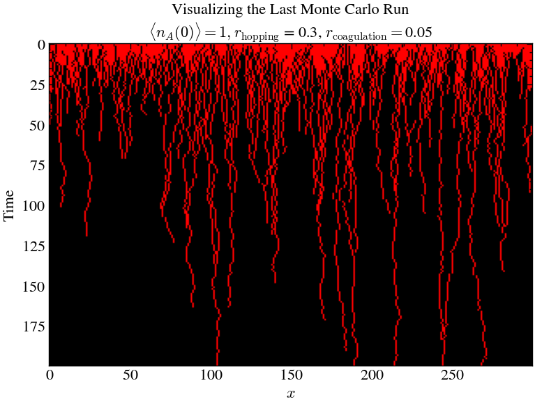

Above shows the time-evolution of Monte-Carlo simulation of the one-dimensional binary-annihilation reaction with periodic boundary conditions. Hopping probability 25% in either direction. Every site in the inital lattice is occupied by a particle.

Theoretically, we can also solve this using differential equations.

\begin{align*} \frac{\partial \langle n_\mathrm{A}(t) \rangle}{\partial t} & = - k \left\langle [ n_\mathrm{A} (n_\mathrm{A} - 1)](t) \right\rangle \approx - k \left\langle n_\mathrm{A}^2 (t) \right\rangle \\ \langle n_\mathrm{A}(t)\rangle = A \, t^{-\alpha} + \epsilon(t) & \implies \boxed{\log \langle n_\mathrm{A}(t)\rangle \propto - \log t} \end{align*}

(2)

# Comparison with differential equation: d[A]/dt = -k[A]
def first_order_reaction(t, y, k):
    return -k * y**2

y0 = [1]
t_span = (0, 200)
t_eval = np.linspace(0, 200, 100)
k1 = 0.5
k2 = 0.07
# Solve using RK45
sol1 = solve_ivp(first_order_reaction, t_span, y0, method='RK45', t_eval=t_eval, args=(k1,))
sol2 = solve_ivp(first_order_reaction, t_span, y0, method='RK45', t_eval=t_eval, args=(k2,))

plt.plot(np.mean(number_densities, axis=0)/L, label='$\\langle n_A \\rangle$')
plt.plot(np.mean(hops_per_step, axis=0), label='$\\langle D \\rangle$')
plt.plot(sol1.t, sol1.y[0], '--', label=f'$\\langle n_A \\rangle$ theoretical, $k =$ {k1}')
plt.plot(sol2.t, sol2.y[0], '--', label=f'$\\langle n_A \\rangle$ theoretical, $k =$ {k2}')
plt.legend()
plt.xlabel('Time Steps [MCS]')
plt.ylabel('Value Density')
plt.title(f'Number density and the Effective Hopping rate over {ntimes} runs')
plt.grid()
plt.yscale('log')
plt.show()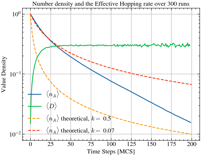

The theoretical value sort of matches with the simulations at the beginning, but quickly deviates. This is beacuse Also, theoretical $\langle n \rangle$ value goes to 0 for large enough values of $k$ here while the simulation does not, due to the formation of isolated islands where the particles can remain stable for a long time -- more likely to happen in a realistic scenario.

Effective hopping rate determination¶

ntimes = 300
_, _, hops_per_step1 = run_coagulation(ntimes, L, T, 0.1, coagulation_rate)
_, _, hops_per_step2 = run_coagulation(ntimes, L, T, 0.2, coagulation_rate)
_, _, hops_per_step3 = run_coagulation(ntimes, L, T, 0.3, coagulation_rate)
_, _, hops_per_step4 = run_coagulation(ntimes, L, T, 0.4, coagulation_rate)

plt.plot(np.mean(hops_per_step1, axis=0), label='$r_\\text{h} = 0.1$')
plt.plot(np.mean(hops_per_step2, axis=0), label='$r_\\text{h} = 0.2$')
plt.plot(np.mean(hops_per_step3, axis=0), label='$r_\\text{h} = 0.3$')
plt.plot(np.mean(hops_per_step4, axis=0), label='$r_\\text{h} = 0.4$')
plt.legend()
plt.xlim(0, 270)
plt.xlabel('Time')
plt.ylabel('$\\langle D \\rangle$')
plt.title(f'Effective Hopping rate over {ntimes} runs')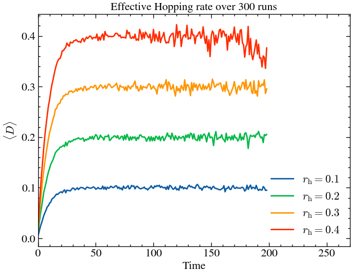

As expected, the hopping probability directly translates to higher number of hops, but in all cases it stabilises after a certain time, due to the formation of islands, as explained previously.

Extension to 2D¶

We can extend the same problem to 2 dimensions.

@njit(parallel=True)
def initialise_world(lattice, species, initial_densities, carrying_capacity=1, uniform_dist=False):
    N = lattice.shape[1]
    # make sure intital _densities are a numpy float64 array
    species_probability = initial_densities/np.sum(initial_densities)

    for x in prange(N):
        for y in prange(N):
            s = weighted_choice(species, species_probability)
            if carrying_capacity == 1:
                lattice[s, x, y] = 1
            else:
                sdensity = initial_densities[s]
                if uniform_dist:
                    lattice[s, x, y] = lattice[s, x, y]+1 if np.random.random() < sdensity else lattice[s, x, y] 
                else:
                    lattice[s,x,y] += np.random.poisson(sdensity)

                if carrying_capacity != None and (np.sum(lattice[:,x,y]) > carrying_capacity):
                    lattice[s,x,y] -= np.sum(lattice[:,x,y])-carrying_capacity
    return lattice

# @njit("Tuple([float64[:,:], f8[:,:], f8[:,:]])(i8,i8,i8,i8[:],float64,float64)",)
@njit
def run_coagulation2d(ntimes, L, T, species_list, initialise_randomly, hopping_rate, coagulation_rate):
    nspecies = len(species_list)
    number_density_average = np.zeros((ntimes, T, nspecies), dtype=np.int32)

    # run the simulation ntimes number of times
    for itime in prange(ntimes):
        world_evolution = np.zeros((T, nspecies, L, L), dtype=np.int32) # world as it evolves
        
        # initialise randomly means non-uniform distribution
        world = initialise_world(np.zeros((nspecies, L, L), dtype=np.int32), species_list, np.array([1.0]), 1, not(initialise_randomly))

        world_evolution[0] = world

        # essentially the same as sum(world, axis=(1,2))
        number_density_average[itime, 0] = np.sum(world, axis=1).sum(axis=1)

        for ti in range(1, T):
            world = world_evolution[ti-1] # previous iteration

            N_per_species = number_density_average[itime, ti-1]
            N = np.sum(N_per_species)
            
            # one monte carlo step
            for nj in range(N):

                # single species annihilation in 2d 
                non_empty_spaces = np.column_stack(np.where(world[0] > 0))
                rx, ry = random_pick(non_empty_spaces)
                rx = -1 if rx==L-1 else rx
                ry = -1 if ry==L-1 else ry # periodic boundary condition

                if np.random.random() < hopping_rate:
                    # pick new location from one of the neighbouring sites

                    possible_hops = []
                    for nx, ny in [(rx+1,ry), (rx-1, ry), (rx,ry+1), (rx,ry-1)]:
                        if world[0][nx, ny] == 0:
                            possible_hops.append((nx, ny))

                    if possible_hops:
                        world[0][rx, ry] -= 1
                        rx, ry = random_pick(possible_hops)
                        world[0][rx, ry] += 1

                if np.random.random() < coagulation_rate:
                    rx = -1 if rx==L-1 else rx
                    ry = -1 if ry==L-1 else ry

                    possible_coagulation_locs = []
                    for nx, ny in [(rx+1,ry), (rx-1, ry), (rx,ry+1), (rx,ry-1)]:
                        if world[0][nx, ny] == 1:
                            possible_coagulation_locs.append((nx, ny))

                    if possible_coagulation_locs:
                        nx, ny = random_pick(possible_coagulation_locs)
                        world[0][nx, ny] -= 1

            world_evolution[ti] = world
            number_density_average[itime, ti] = np.sum(world, axis=1).sum(axis=1)

    # return the last world_evolution array (only for visualisation purposes)
    return world_evolution, number_density_average

L,T = 100,500
ntimes = 5
hopping_rate = 0.3
coagulation_rate = 0.05
world_evolution, number_densities = run_coagulation2d(ntimes, L, T, [0], False, hopping_rate, coagulation_rate)

# number_densities[ntimes, T, nspecies]
for i in range(ntimes):
    plt.plot(number_densities[i, :, 0]/L**2, 'r', alpha=0.1)
plt.plot(number_densities.mean(axis=0)[:,0]/L**2, 'r', alpha=1)
plt.xlim(0,T)
plt.yscale('log')
plt.xlabel('Time [MCS]')
plt.grid()
plt.ylabel('$\\langle n \\rangle$')
plt.title('Single Species Annihilation\nNumber Density Evolution')
plt.show()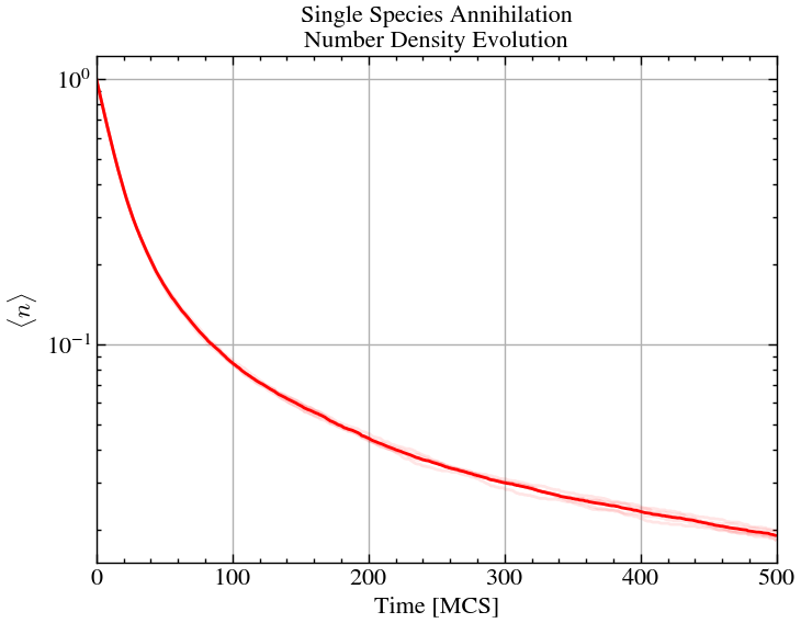

fig, ax = plt.subplots(figsize=(6,6))
def animate(i, title):
    ax.clear()
    a = ax.imshow(world_evolution[i, 0])#, cmap=plt.get_cmap('inferno'))
    ax.set_title(f'{title}\nMCS = {i:2}')
    ax.set_xticks([]) 
    ax.set_yticks([]) 
    return fig,

title = '2D Single Species Annihilation\n(w/ Uniform Inital Density)'
a = ax.imshow(world_evolution[0, 0])
ani = animation.FuncAnimation(fig, animate, frames=T, interval=50, blit=True, fargs=(title,))
ani.save('animations/2d_coagulation.gif',writer='pillow',fps=20)

HTML(ani.to_html5_video())

Double Species Annihilation¶

They are reactions where two different particles meet and annihilate each other.

A + B \rightarrow \phi

(3)

@njit
def binary_species_annihilation(world, loc, *params):
    hopping_rate = params[0]
    species_picked = world[loc]
    hops = 0

    to_hop_or_not_to_hop = np.random.random()
    if to_hop_or_not_to_hop < hopping_rate[species_picked]:

        if world[loc-1] == -1:
            world[loc-1] = species_picked
            world[loc] = -1
            hops += 1

        elif (species_picked == 1 and world[loc-1] == 0) or (species_picked == 0 and world[loc-1] == 1):
            world[loc - 1], world[loc] = -1, -1
            hops += 1
            
    elif to_hop_or_not_to_hop < hopping_rate[species_picked]*2: # assuming right and left hopping rates are equal
        loc = -1 if loc == L-1 else loc

        if world[loc+1] == -1:
            world[loc+1] = species_picked
            world[loc] = -1
            hops += 1
        elif (species_picked == 1 and world[loc+1] == 0) or (species_picked == 0 and world[loc+1] == 1):
            world[loc + 1], world[loc] = -1, -1
            hops += 1

    return world, hops

with non-uniform inital field¶

L, T = 300, 250
hopping_rate = [0.25, 0.25]
ntimes = 100
world_evolution_last, number_densities, hops_per_step = run_coagulation(binary_species_annihilation, ntimes, L, T, [0,1], True, hopping_rate)
number_densities /= L**2

xi = np.arange(0,L)
yi = np.arange(0,T)
xi, yi = np.meshgrid(xi, yi)

plt.figure(figsize=(12, 6))
cmap = ListedColormap(['k', 'r', 'b'])
plt.imshow(world_evolution_last, cmap=cmap, origin='lower')
plt.xlabel('$x$')
plt.ylabel('Time')
plt.title('Binary Annihilation\nw/ Random Inital Configuration')
plt.gca().invert_yaxis()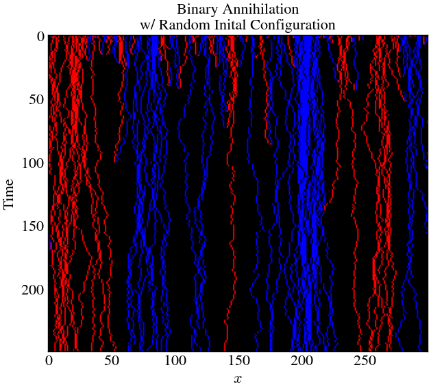

Here, we see significant island formation for A and B. This is because there were small clusters of same particles, formed non-uniformly early on, which remained relatively stable over time. Essentially, they all protected each other from annihilation.

averaged_n = number_densities.mean(axis=0).transpose()
for i in range(ntimes):
    plt.plot(number_densities[i, :, 0], 'r', alpha=0.04)
    plt.plot(number_densities[i, :, 1], 'b', alpha=0.04)
n_species0 = averaged_n[0]
n_species1 = averaged_n[1]
plt.plot(n_species0, 'b', label='$\\langle n_\\text{A} \\rangle$')
plt.plot(n_species1, 'r', label='$\\langle n_\\text{B} \\rangle$')
plt.legend()
plt.ylim(1e-4,np.max(number_densities))
plt.xlim(-1, T)
plt.xlabel('Time Steps [MCS]')
plt.ylabel('Number Density')
plt.title(f'Number density over {ntimes} runs')
plt.yscale('log')

with uniform inital field¶

L, T = 300, 250
hopping_rate = [0.25, 0.25]
world_evolution_last, number_densities, hops_per_step = run_coagulation(binary_species_annihilation, 100, L, T, [0,1], False, hopping_rate)
number_densities /= L**2

xi = np.arange(0,L)
yi = np.arange(0,T)
xi, yi = np.meshgrid(xi, yi)

plt.figure(figsize=(12, 6))
cmap = ListedColormap(['k', 'r', 'b'])
plt.imshow(world_evolution_last, cmap=cmap, origin='lower')
plt.xlabel('$x$')
plt.ylabel('Time')
# plt.ylim(0,5)
plt.gca().invert_yaxis()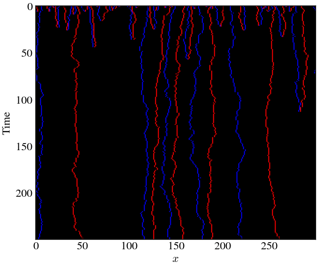

As expected, for the uniform inital field, the formation of islands are less significant since there was a higher chance of different particles meeting each other early on as the field was uniformly distributed.

averaged_n = number_densities.mean(axis=0).transpose()
for i in range(ntimes):
    plt.plot(number_densities[i, :, 0], 'r', alpha=0.01)
    plt.plot(number_densities[i, :, 1], 'b', alpha=0.01)
n_species0 = averaged_n[0]
n_species1 = averaged_n[1]
plt.plot(n_species0, 'b', label='$\\langle n_\\text{A} \\rangle$')
plt.plot(n_species1, 'r', label='$\\langle n_\\text{B} \\rangle$')
plt.legend()
plt.xlim(-1, T)
plt.xlabel('Time Steps [MCS]')
plt.ylabel('Number Density')
plt.title(f'Number density over {ntimes} runs')
plt.yscale('log')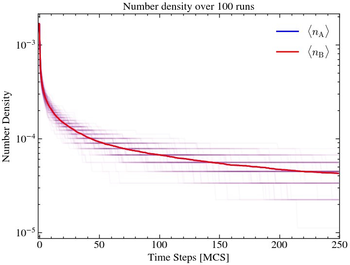

Extension to 2D¶

We can also extend this to 2 dimensions (w/ Inital Possion Density)

@njit
def run_binary_annihilation2d(ntimes, L, T, species_list, initialise_randomly, hopping_rate):
    nspecies = len(species_list)
    number_density_average = np.zeros((ntimes, T, nspecies), dtype=np.int32)

    # run the simulation ntimes number of times
    for itime in prange(ntimes):
        world_evolution = np.zeros((T, nspecies, L, L), dtype=np.int32) # world as it evolves
        
        # initialise randomly means non-uniform distribution
        world = initialise_world(np.zeros((nspecies, L, L), dtype=np.int32), species_list, np.array([1.0, 1.0]), 1, not(initialise_randomly))

        world_evolution[0] = world

        # essentially the same as sum(world, axis=(1,2))
        number_density_average[itime, 0] = np.sum(world, axis=1).sum(axis=1)

        for ti in range(1, T):
            world = world_evolution[ti-1] # previous iteration

            N_per_species = number_density_average[itime, ti-1]
            N = np.sum(N_per_species)
            
            # one monte carlo step
            for nj in range(N):

                # binary species annihilation in 2d 
                if np.random.random() < N_per_species[0]/N:
                    species_picked = 0
                    other_speciess = 1
                else:
                    species_picked = 1
                    other_speciess = 0

                non_empty_spaces = np.column_stack(np.where(world[species_picked] > 0))
                rx, ry = random_pick(non_empty_spaces)
                rx = -1 if rx==L-1 else rx
                ry = -1 if ry==L-1 else ry # periodic boundary condition

                if np.random.random() < hopping_rate:
                    # pick new location from one of the neighbouring sites

                    possible_hops = []
                    for nx, ny in [(rx+1,ry), (rx-1, ry), (rx,ry+1), (rx,ry-1)]:
                        if world[species_picked][nx, ny] == 0:
                            possible_hops.append((nx, ny))

                    if possible_hops:
                        world[species_picked][rx, ry] -= 1
                        rx, ry = random_pick(possible_hops)
                        world[species_picked][rx, ry] += 1

                if np.random.random() < coagulation_rate:
                    rx = -1 if rx==L-1 else rx
                    ry = -1 if ry==L-1 else ry

                    possible_coagulation_locs = []
                    for nx, ny in [(rx+1,ry), (rx-1, ry), (rx,ry+1), (rx,ry-1)]:
                        if world[other_speciess][nx, ny] == 1:
                            possible_coagulation_locs.append((nx, ny))

                    if possible_coagulation_locs:
                        nx, ny = random_pick(possible_coagulation_locs)
                        world[other_speciess][nx, ny] -= 1
                        world[species_picked][rx, ry] -= 1

            world_evolution[ti] = world
            number_density_average[itime, ti] = np.sum(world, axis=1).sum(axis=1)

    # return the last world_evolution array (only for visualisation purposes)
    return world_evolution, number_density_average

L,T = 100,500
ntimes = 1
hopping_rate = 0.3
coagulation_rate = 0.05
world_evolution, number_densities = run_binary_annihilation2d(ntimes, L, T, [0,1], False, hopping_rate)

fig, ax = plt.subplots(figsize=(6,6))

def animate(ti, title):
    ax.clear()
    image = np.zeros((L, L, 3), dtype=np.uint8)
    image[:, :, 0] = 255*(world_evolution[ti, 0])
    image[:, :, 2] = 255*(world_evolution[ti, 1])
    ax.imshow(image)
    ax.set_title(f'{title}\nMCS = {ti:2}')
    ax.set_xticks([]) 
    ax.set_yticks([]) 
    return fig,

title = '2D Binary Species Annihilation'
ani = animation.FuncAnimation(fig, animate, frames=T, interval=50, blit=True, fargs=(title,))
ani.save('animations/2d_binary_annihilation_non_uniform.gif',writer='pillow',fps=20)

HTML(ani.to_html5_video())

Here, the red and blue represent A and B particles and pink represents locations in the lattice where both A and B are present.

averaged_n = number_densities.mean(axis=0).transpose()
for i in range(ntimes):
    plt.plot(number_densities[i, :, 0], 'r', alpha=0.04)
    plt.plot(number_densities[i, :, 1], 'b', alpha=0.04)
n_species0 = averaged_n[0]
n_species1 = averaged_n[1]
plt.plot(n_species0, 'b', label='$\\langle n_\\text{A} \\rangle$')
plt.plot(n_species1, 'r', label='$\\langle n_\\text{B} \\rangle$')
plt.legend()
plt.ylim(np.min(number_densities),np.max(number_densities))
plt.xlim(-1, T)
plt.xlabel('Time Steps [MCS]')
plt.ylabel('Number Density')
plt.title(f'2D Binary Annihilation Reaction w/Non-uniform inital config\nNumber density over {ntimes} run(s)')
plt.yscale('log')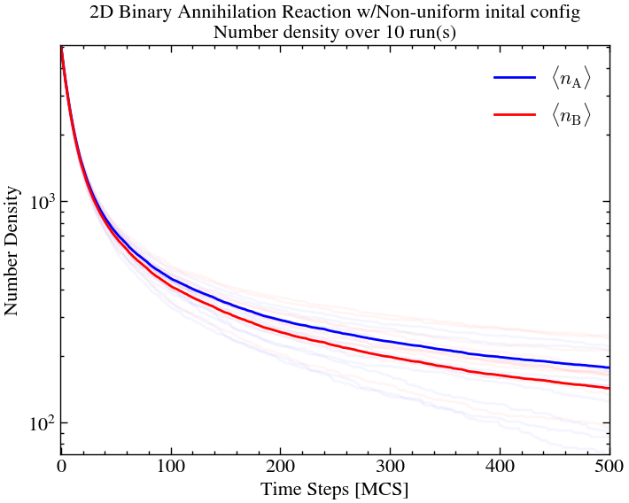

Now, we do the same thing but withour uniform inital configuration.

world_evolution_uniform, number_densities_uniform = run_binary_annihilation2d(ntimes, L, T, [0,1], True, hopping_rate)

fig, ax = plt.subplots(figsize=(6,6))

def animate(ti, title):
    ax.clear()
    image = np.zeros((L, L, 3), dtype=np.uint8)
    image[:, :, 0] = 255*(world_evolution_uniform[ti, 0])
    image[:, :, 2] = 255*(world_evolution_uniform[ti, 1])
    ax.imshow(image)
    ax.set_title(f'{title}\nMCS = {ti:2}')
    ax.set_xticks([]) 
    ax.set_yticks([]) 
    return fig,

title = '2D Binary Species Annihilation'
ani = animation.FuncAnimation(fig, animate, frames=T, interval=50, blit=True, fargs=(title,))
ani.save('animations/2d_binary_annihilation_uniform.gif',writer='pillow',fps=20)

HTML(ani.to_html5_video())

averaged_n = number_densities_uniform.mean(axis=0).transpose()
for i in range(ntimes):
    plt.plot(number_densities_uniform[i, :, 0], 'r', alpha=0.04)
    plt.plot(number_densities_uniform[i, :, 1], 'b', alpha=0.04)
n_species0 = averaged_n[0]
n_species1 = averaged_n[1]
plt.plot(n_species0, 'b', label='$\\langle n_\\text{A} \\rangle$')
plt.plot(n_species1, 'r', label='$\\langle n_\\text{B} \\rangle$')
plt.legend()
plt.ylim(np.min(number_densities_uniform),np.max(number_densities_uniform))
plt.xlim(-1, T)
plt.xlabel('Time Steps [MCS]')
plt.ylabel('Number Density')
plt.title(f'2D Binary Annihilation Reaction (w/ Non-uniform inital config)\nNumber density over {ntimes} run(s)')
plt.yscale('log')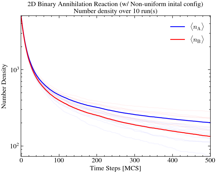

On comparison, we see that the uniform and non-uniform initial fields essentially over 10 iterations amount to the same thing. This is the advantage of more dimensions, offering the particles more degrees of freedom.

averaged_n = number_densities_uniform.mean(axis=0).transpose()
plt.plot(n_species0, 'b', label='$\\langle n_\\text{A} \\rangle$ (U)')
plt.plot(n_species1, 'r', label='$\\langle n_\\text{B} \\rangle$ (U)')
averaged_n = number_densities.mean(axis=0).transpose()
plt.plot(n_species0, 'b--', label='$\\langle n_\\text{A} \\rangle$ (NU)')
plt.plot(n_species1, 'r--', label='$\\langle n_\\text{B} \\rangle$ (NU)')
plt.legend()
plt.ylim(np.min(number_densities_uniform),np.max(number_densities_uniform))
plt.xlim(-1, T)
plt.xlabel('Time Steps [MCS]')
plt.ylabel('Number Density')
plt.title(f'2D Binary Annihilation Reaction\nNumber density over {ntimes} run(s)')
plt.yscale('log')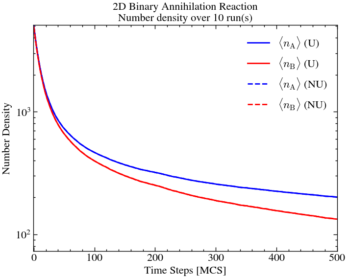

# np.savez_compressed('data/binary', nonuni=world_evolution, uni=world_evolution_uniform)
# world_evolution = np.load('data/LV2.npz', allow_pickle=True )['nonuni']

2D Correlation Function¶

This essentially measures the frequency of distance between two particles of the same species. It is a good tool to assess/quantify the rate of clumping in a 2D lattice.

@njit
def measure_2d_distance(given_matrix):
    matrix = given_matrix.copy()
    distances = []
    for (ix, iy), vali in np.ndenumerate(matrix):
        if vali == 1:
            for (jx, jy), valj in np.ndenumerate(matrix):
                if valj == 1 and ix!=jx and iy!=jy:
                    distances.append(np.sqrt((ix-jx)**2+(iy-jy)**2))
        matrix[ix, iy] = 0
        
    return distances

For Non-uniform inital field¶

plt.figure(figsize=(12, 6))
plt.subplot(121)
plt.hist(measure_2d_distance(world_evolution[5, 0]), 20,histtype='step',linewidth=3, color='b',density=True)
plt.hist(measure_2d_distance(world_evolution[5, 1]), 20,histtype='step',linewidth=3, color='r',density=True)
plt.xlabel('Distance')
plt.ylabel('Frequency')
plt.title('2D correlation measured \nat MCS = 5')
plt.subplot(122)
plt.hist(measure_2d_distance(world_evolution[-1, 0]), 20,histtype='step',linewidth=3, color='b', label='A',density=True)
plt.hist(measure_2d_distance(world_evolution[-1, 1]), 20,histtype='step',linewidth=3, color='r', label='B',density=True)
plt.xlabel('Distance')
# plt.ylabel('Frequency')
plt.legend()
plt.title('2D correlation measured \nat MCS = 499')
plt.show()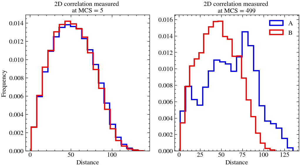

For Uniform inital field¶

plt.figure(figsize=(12, 6))
plt.subplot(121)
plt.hist(measure_2d_distance(world_evolution_uniform[5, 0]), 20,histtype='step',linewidth=3, color='b',density=True)
plt.hist(measure_2d_distance(world_evolution_uniform[5, 1]), 20,histtype='step',linewidth=3, color='r',density=True)
plt.xlabel('Distance')
plt.ylabel('Frequency')
plt.title('2D correlation measured \nat MCS = 5')
plt.subplot(122)
plt.hist(measure_2d_distance(world_evolution_uniform[-1, 0]), 20,histtype='step',linewidth=3, color='b', label='A',density=True)
plt.hist(measure_2d_distance(world_evolution_uniform[-1, 1]), 20,histtype='step',linewidth=3, color='r', label='B',density=True)
plt.xlabel('Distance')
# plt.ylabel('Frequency')
plt.legend()
plt.title('2D correlation measured \nat MCS = 499')
plt.show()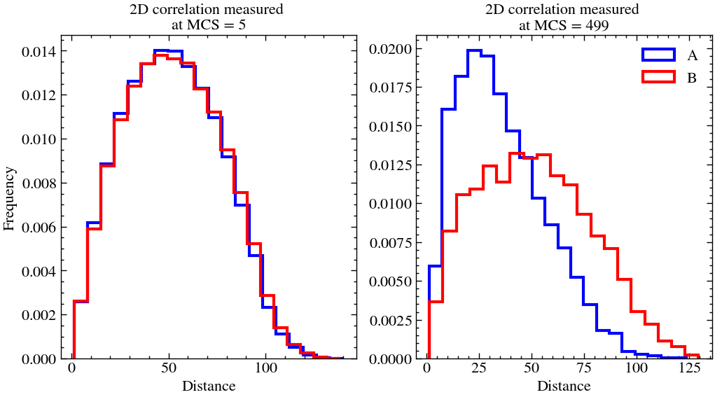

As one can see, in both the cases, we start of with the histogram fairly being a bell curve with maximum frequency around 50, which half of the lattice size. But as time progresses, in the last snapshot, we can observe that the initally uniform lattice is more clumped (not by much) since the histogram is skewed more towards lower distances. This can also be verified by visualising the last snapshot.

plt.figure(figsize=(12, 6))
plt.subplot(121)
image = np.zeros((L, L, 3), dtype=np.uint8)
image[:, :, 0] = 255*(world_evolution[-1, 0])
image[:, :, 2] = 255*(world_evolution[-1, 1])
plt.imshow(image)
plt.title(f'Uniform Intial Config Snapshot\nMCS = {499:2}')
plt.gca().set_xticks([]) 
plt.gca().set_yticks([]) 
plt.subplot(122)
image = np.zeros((L, L, 3), dtype=np.uint8)
image[:, :, 0] = 255*(world_evolution_uniform[-1, 0])
image[:, :, 2] = 255*(world_evolution_uniform[-1, 1])
plt.imshow(image)
plt.title(f'Non-Uniform Intial Config Snapshot\nMCS = {499:2}')
plt.gca().set_xticks([]) 
plt.gca().set_yticks([]) 
plt.show()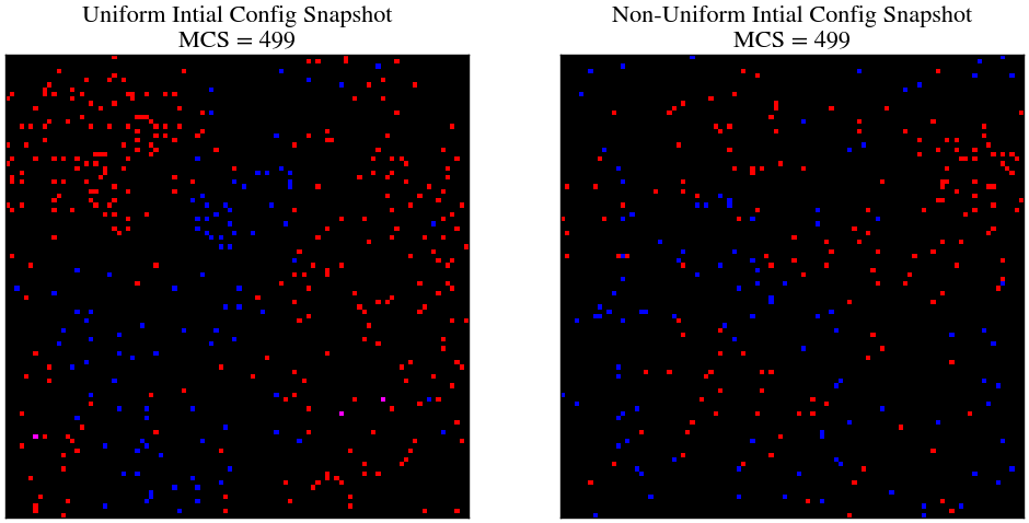

Hence, we have visually verified the correctness of the correlation function. This is one of the ways you can use Monte-Carlo simulations to assess spatial structures which are purely a result of stocasticity and probabilistic reaction equations.

Predator-Prey Models¶

Let us look at the dynamics of a simple 2D Lotka-Volterra Prey-Predator Model. The dynamics of the world are represented by,

\begin{align*} \mathrm{Prey} + \mathrm{Predator} & \xrightarrow{r_{predation}} 2\mathrm{ Predator}\\ \mathrm{Prey} & \xrightarrow{r_b} 2\mathrm{ Prey}\\ \mathrm{Predator} & \xrightarrow{r_d} \phi \end{align*}

(4)

Spontaneous Structure Formation¶

@njit
def run_prey_predator(ntimes, L, T, species_list, inital_density, hopping_rates, predation_rate, predator_death_rate, prey_birth_rate, progress_proxy):
    prey, predator = species_list
    nspecies = len(species_list)
    number_density_average = np.zeros((ntimes, T, nspecies), dtype=np.int64)

    # run the simulation ntimes number of times
    for itime in prange(ntimes):
        i = 0
        world_evolution = np.zeros((T, nspecies, L, L), dtype=np.int64) # world as it evolves
        
        # initialise randomly means non-uniform distribution
        world = initialise_world(np.zeros((nspecies, L, L)), species_list, inital_density, None)

        world_evolution[0] = world

        # essentially the same as sum(world, axis=(1,2))
        number_density_average[itime, 0] = np.sum(world, axis=1).sum(axis=1)

        for ti in range(1, T):
            world = world_evolution[ti-1] # previous iteration

            N_per_species = number_density_average[itime, ti-1]
            N = np.sum(N_per_species)
            N_probs = N_per_species/N
            
            # one monte carlo step
            for nj in range(N):

                species_picked = weighted_choice(species_list, N_probs)
                # print()
                non_empty_spaces = np.column_stack(np.where(world[species_picked] > 0))
                
                if non_empty_spaces.shape[0] == 0:
                    break

                rx, ry = random_pick(non_empty_spaces)
                rx = -1 if rx==L-1 else rx
                ry = -1 if ry==L-1 else ry # periodic boundary condition

                if np.random.random() < hopping_rates[species_picked]:
                    world[species_picked][rx, ry] -= 1
                    nx, ny = random_pick([(rx+1,ry), (rx-1, ry), (rx,ry+1), (rx,ry-1)])
                    world[species_picked][nx, ny] += 1
                
                if species_picked == prey:
                    if np.random.random() < prey_birth_rate:
                        world[prey][rx, ry] += 1

                elif species_picked == predator:
                    # print(f'predator at {}')
                    vulnerable_preys = world[prey][rx,ry]
                    for _ in range(vulnerable_preys):
                        if np.random.random() < predation_rate:
                            world[prey][rx, ry] -= 1
                            world[predator][rx, ry] += 1

                    if np.random.random() < predator_death_rate:
                        world[predator][rx, ry] -= 1

            world_evolution[ti] = world
            number_density_average[itime, ti] = np.sum(world, axis=1).sum(axis=1)

        progress_proxy.update(1)
    # return the last world_evolution array (only for visualisation purposes)
    return world_evolution, number_density_average

initial_densities = np.array([1.0, 0.005])
prey = 0
predator = 1

species = [prey, predator]
hopping_rates = [1.0, 1.0]

# lambda, mu, sigma in the paper respectively
predation_rate, predator_death_rate, prey_birth_rate = 0.1, 0.1, 0.1

L,T = 100, 300
ntimes = 5
with ProgressBar(total=ntimes) as progress:
    world_evolution_lv, number_densities_lv = run_prey_predator(ntimes, L, T, species, initial_densities, hopping_rates, predation_rate, predator_death_rate, prey_birth_rate)

plt.plot(number_densities_lv[0,:, 0]/L**2, 'b', label='Prey')
plt.plot(number_densities_lv[0,:, 1]/L**2, 'r', label='Predator')
plt.xlabel('Time Steps [MCS]')
plt.ylabel('Number Density [occupants/site]')
plt.title('Lotka-Volterra Model w/\n $r_\\text{predation} =$ ' + str(predation_rate) + '$, r_\\text{d, predator}=$' + str(predator_death_rate) + '$, r_\\text{b, prey}=$' + str(prey_birth_rate))
plt.legend()
plt.xlim(0, T)
plt.show()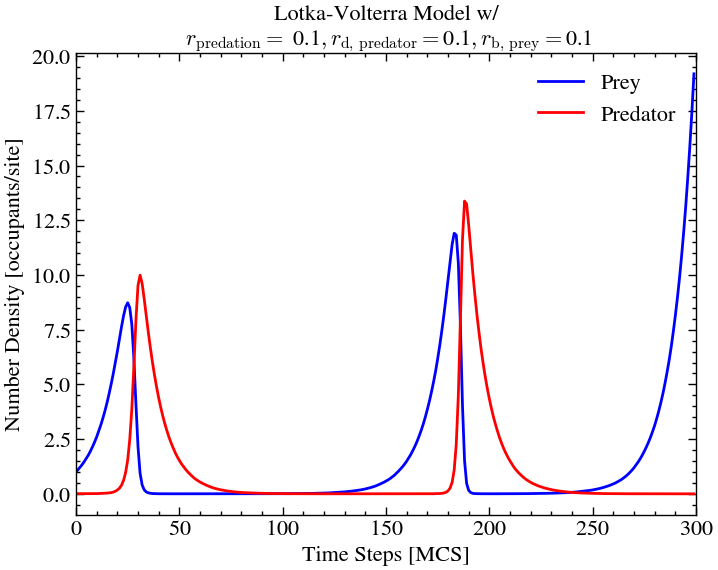

Note: This is the result of a single Monte-Carlo simulation. Here, we have not performed a large number of simulations. Due to the complexity of the problem, it would take a huge amount of computational time to compute that.

So, it is possible that in some cases, we do not see the second wave because all the preys died out due to the stochastic nature of the simulation.

fig, ax = plt.subplots(figsize=(6,7))

def animate(ti, title):
    ax.clear()
    image = np.zeros((L, L, 3), dtype=np.uint8)
    image[:, :, 0] = 255*(world_evolution_lv[ti, 1]) # R -> predator
    image[:, :, 2] = 255*(world_evolution_lv[ti, 0]) # B -> prey
    ax.imshow(image)
    ax.set_title(f'{title}\nMCS = {ti:2}')
    ax.set_xticks([]) 
    ax.set_yticks([]) 
    return fig,

title = 'Lotka-Volterra Model w/\n $r_\\text{predation} =$ ' + str(predation_rate) + '$, r_\\text{d, predator}=$' + str(predator_death_rate) + '$, r_\\text{b, prey}=$' + str(prey_birth_rate)
ani = animation.FuncAnimation(fig, animate, frames=T, interval=50, blit=True, fargs=(title,))
ani.save('animations/LV2.gif',writer='pillow',fps=20)

HTML(ani.to_html5_video())

Here, the red and blue represent predator and prey particles respectively and pink represents locations in the lattice where both are present.

A story in four parts -- why we need Monte-Carlo simulations¶

The following code will only work for this particular simulation. To see an example of a classic prey-predator scenario, consider the following snapshots. We begin with very few prey particles scattered evenly. As time evolves, we see these few predator particles reproduce rapidly as they flourish in an area abundant with prey. This induces local population expansion of the predator particles, as seen in the second image. Now, the Prey are rapidly consumed which leaves a region of low abundance in which the predator cannot survive for long (3rd image), this causes them to deplete fast. Now, there are some empty spaces in the lattice, where some (very few) prey particles survived miraculously. Over time, these prey particles can now replenish, thus we go back to square one. This nontrivial persistent wave front dynamics can only be observed in Monte-Carlo simulations of the Lotka–Volterra model, since random population oscillations are necessary for these kind of behavior. Wuch behavious cannot be explained by using simple differential equations.

plt.figure(figsize=(15,10))
plt.subplot(141)
image = np.zeros((L, L, 3), dtype=np.uint8)
image[:, :, 0] = 255*(world_evolution_lv[7, 1])
image[:, :, 2] = 255*(world_evolution_lv[7, 0])
plt.title('MCS = 7')
plt.imshow(image)
plt.subplot(142)
image = np.zeros((L, L, 3), dtype=np.uint8)
image[:, :, 0] = 255*(world_evolution_lv[24, 1])
image[:, :, 2] = 255*(world_evolution_lv[24, 0])
plt.title('MCS = 24')
plt.imshow(image)
plt.subplot(143)
image = np.zeros((L, L, 3), dtype=np.uint8)
image[:, :, 0] = 255*(world_evolution_lv[34, 1]) 
image[:, :, 2] = 255*(world_evolution_lv[34, 0])
plt.title('MCS = 34')
plt.imshow(image)
plt.subplot(144)
image = np.zeros((L, L, 3), dtype=np.uint8)
image[:, :, 0] = 255*(world_evolution_lv[71, 1]) 
image[:, :, 2] = 255*(world_evolution_lv[71, 0])
plt.title('MCS = 71')
plt.imshow(image)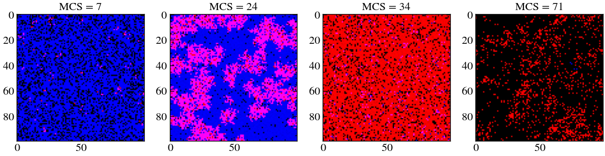

# np.savez_compressed('data/LV2', numbers=world_evolution_lv)
# world_evolution_lv = np.load('data/LV2.npz', allow_pickle=True )['numbers']

Autocorrelation¶

Autocorrelation function basically aims to quantify stucture formation, by calculating the distance between every particle of a certain species. Here, we have used predator particles for the same. Note that in the simulation, when certain waves break out, the frequency of smaller distances increase significantly.

@njit(nogil=True)
def measure_auto_correlation(L, given_matrix):
    matrix = given_matrix.copy()
    distances = []

    for (ix, iy), vali in np.ndenumerate(matrix):
        if vali > 0:
            for _ in range(vali-1): # distance 0
                distances.append(0)
            
            for (jx, jy), valj in np.ndenumerate(matrix):
                if valj > 0 and ix!=jx and iy!=jy:
                    dis_ij = np.sqrt((ix-jx)**2+(iy-jy)**2)
                    for _ in range(valj):
                        distances.append(dis_ij)
        matrix[ix, iy] = 0
        
    return distances

predator_distances = []
cleave = 2
for ti in range(0, T, 5):
    predator_distance = measure_auto_correlation(L//cleave, world_evolution_lv[ti, 1, ::cleave, ::cleave])
    predator_distances.append(predator_distance)

fig, ax = plt.subplots(figsize=(8,6))

def animate(ti, title):
    ax.clear()
    ax.hist(predator_distances[ti], bins=20, density=1)
    ax.set_title(f'{title}\nMCS = {ti*5:2}')
    ax.set_xlabel('Distance')
    ax.set_ylabel('Normalised Frequency')
    return fig,

title = 'Lotka-Volterra Model\nPredator Auto-Correlation'
ani = animation.FuncAnimation(fig, animate, frames=300//5, interval=50, blit=True, fargs=(title,))
ani.save('animations/LV_Predator_AutoCorr.gif',writer='pillow',fps=20)

HTML(ani.to_html5_video())

Picking out low autocorrelation¶

In the above animation, one can see, for example, that at $MCS=230$ , the histogram is quite skewed in towards lower numbers. Let us investigate that.

Note: Here, we have manually picked a time snapshot from the above animation where the autocorrelation function was relatively skewed. This most likely will not work for a different simulation.

mcs1 = 230
hist1 = measure_auto_correlation(L//cleave, world_evolution_lv[mcs1, 1, ::cleave, ::cleave])

f, (a0, a1) = plt.subplots(1, 2, figsize=(12,4), gridspec_kw={'width_ratios': [2, 1]})
a0.hist(hist1, bins=20, density=1)
a0.set_xlabel('Distance')
a0.set_ylabel('Normalised Frequency')
a0.set_title(f'Predator Auto-Correlation\nMCS={mcs1}')
image = np.zeros((L, L, 3), dtype=np.uint8)
image[:, :, 0] = 255*(world_evolution_lv[mcs1, 1]) # R -> predator
image[:, :, 2] = 255*(world_evolution_lv[mcs1, 0])
a1.imshow(image)
a1.set_xticks([])
a1.set_yticks([])
a1.set_title('Corresponding World')
plt.show()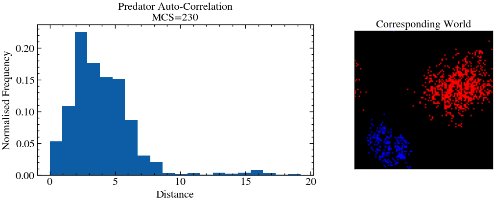

This is an example of structure formation. Predator and prey particles will naturally clump to each other periodically as each wave of predation breaks out, as we saw in the oscillating graph of number densitites. For more uniform distributions, the autocorrelation function will be spread out more. Here we have only calculated the predator autocorrelation since they most likely will be lesser in number and hence will be more efficient to calculate. One can do the same thing to find the prey autocorrelation function.

Epidemic Spreading¶

The susceptible-infectious-recovered (SIR) model is a simplified model for epidemic spreading with recovery/death. The population is divided into -- infected, susceptible, recovered (who are more immune to re-infection than suscptible folk) and dead species. The dynamics of the world is represented by,

\begin{align*} \mathrm{\color{red} I} + \mathrm{\color{blue} S} & \xrightarrow{r_i} \mathrm{\color{red} I} +\mathrm{\color{red} I} \\ \mathrm{\color{red} I} & \xrightarrow{r_r} \mathrm{\color{green} R}\\ \mathrm{\color{green} R} +\mathrm{\color{red} I} & \xrightarrow{r_{ri} \le r_i} \mathrm{\color{red} I}+\mathrm{\color{red} I}\\ \mathrm{\color{red} I} & \xrightarrow{r_{d}} \phi \end{align*}

(5)

@njit(nogil=True)
def run_SIR(ntimes, L, T, species_list, inital_density, infection_rate, recovery_rate,reinfection_rate, death_rate, progress_proxy):
    susceptible, infected, recovered, dead = species_list
    nspecies = len(species_list)
    number_density_average = np.zeros((ntimes, T, nspecies), dtype=np.int64)

    # run the simulation ntimes number of times
    for itime in prange(ntimes):
        world_evolution = np.zeros((T, nspecies, L, L), dtype=np.int64) # world as it evolves
        
        # initialise randomly means non-uniform distribution
        world = initialise_world(np.zeros((nspecies, L, L), dtype=np.int64), species_list, inital_density, 1, True)

        world_evolution[0] = world

        # essentially the same as sum(world, axis=(1,2))
        number_density_average[itime, 0] = np.sum(world, axis=1).sum(axis=1)

        for ti in range(1, T):
            world = world_evolution[ti-1] # previous iteration

            N_per_species = number_density_average[itime, ti-1]
            N = np.sum(N_per_species)
            N_probs = N_per_species/N
            
            # one monte carlo step
            for nj in range(N):

                # binary species annihilation in 2d 
                species_picked = weighted_choice(species_list, N_probs)

                non_empty_spaces = np.column_stack(np.where(world[species_picked] > 0))
                rx, ry = random_pick(non_empty_spaces)
                rx = -1 if rx==L-1 else rx
                ry = -1 if ry==L-1 else ry # periodic boundary condition

                if species_picked == susceptible: # aka susceptible
                    if np.random.random() < infection_rate:
                        # if.shape any of the neighbouring cells are infected, then S gets infected with a certain probability
                        for nx, ny in [(rx+1,ry), (rx-1, ry), (rx,ry+1), (rx,ry-1)]:
                            if world[1][nx, ny] == 1:
                                world[susceptible][rx, ry] = 0
                                world[infected][rx, ry] = 1

                if species_picked == infected:
                    if np.random.random() < recovery_rate:
                        world[infected][rx, ry] = 0
                        world[recovered][rx, ry] = 1

                    if np.random.random() < death_rate:
                        world[infected][rx, ry] = 0
                        world[dead][rx, ry] = 1

                if species_picked == recovered:
                    if np.random.random() < reinfection_rate:
                        # if any of the neighbouring cells are infected, then R gets re-infected with a certain probability < infection_rate
                        for nx, ny in [(rx+1,ry), (rx-1, ry), (rx,ry+1), (rx,ry-1)]:
                            if world[1][nx, ny] == 1:
                                world[recovered][rx, ry] = 0
                                world[infected][rx, ry] = 1

            world_evolution[ti] = world
            number_density_average[itime, ti] = np.sum(world, axis=1).sum(axis=1)
        
        progress_proxy.update(1)

    # return the last world_evolution array (only for visualisation purposes)
    return world_evolution, number_density_average

SIR Model with high transmissivity¶

initial_densities = np.array([1.0, 0.001, 0.0, 0.0])
susceptible = 0
infected = 1
recovered = 2
dead = 3

species = [susceptible, infected, recovered, dead]
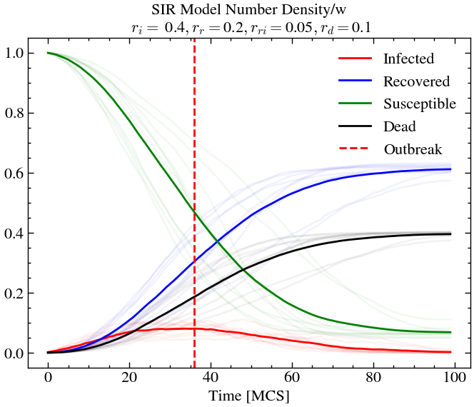
infection_rate, recovery_rate, reinfection_rate, death_rate = 0.4, 0.2, 0.05, 0.1

L,T = 75,100
ntimes = 10
with ProgressBar(total=ntimes) as progress:
    world_evolution_sir, number_densities_sir = run_SIR(ntimes, L, T, species, initial_densities, infection_rate, recovery_rate, reinfection_rate, death_rate, progress)

def plot_sir(number_densities_sir,infection_rate, recovery_rate, reinfection_rate, death_rate,individual_alpha=0.1):
    number_densities_sir = number_densities_sir/L**2
    for itime in range(number_densities_sir.shape[0]):
        plt.plot(number_densities_sir[itime, :, infected], 'r', alpha=individual_alpha)
        plt.plot(number_densities_sir[itime, :, recovered], 'b', alpha=individual_alpha)
        plt.plot(number_densities_sir[itime, :, susceptible], 'g', alpha=individual_alpha)
        plt.plot(number_densities_sir[itime, :, dead], 'k', alpha=individual_alpha)
    n_avg = number_densities_sir.mean(axis=0).transpose()
    plt.plot(n_avg[infected], 'r', label='Infected')
    plt.plot(n_avg[recovered], 'b', label='Recovered')
    plt.plot(n_avg[susceptible], 'g', label='Susceptible')
    plt.plot(n_avg[dead], 'k', label='Dead')
    plt.xlabel('Number density [occupants/site]')
    plt.xlabel('Time [MCS]')
    plt.title(f'SIR Model Number Density/w\n $r_i =$ ' + str(infection_rate) + '$, r_{r}=$' + str(recovery_rate) + '$, r_{ri}=$' + str(reinfection_rate) + '$, r_{d}=$' + str(death_rate))
    plt.axvline(np.argmax(n_avg[infected]), color='r', linestyle='--', label='Outbreak')
    plt.legend()
    return n_avg

# save the results if needed
# np.savez_compressed('data/sir1', world=world_evolution_sir, numbers=number_densities_sir)
# world_evolution_lv = np.load('data/LV2.npz', allow_pickle=True )['numbers']

n_avg = plot_sir(number_densities_sir, infection_rate, recovery_rate, reinfection_rate, death_rate, 0.05)

fig, ax = plt.subplots(figsize=(7,6))

def animate(ti, title):
    ax.clear()
    image = np.zeros((L, L, 3), dtype=np.uint8)
    image[:, :, 0] = 255*(world_evolution_sir[ti, 1]) # R -> infected
    image[:, :, 1] = 255*(world_evolution_sir[ti, 0]) # G -> susceptible
    image[:, :, 2] = 255*(world_evolution_sir[ti, 2]) # B -> recovered
    ax.imshow(image)
    ax.set_title(f'{title}\nMCS = {ti:2}')
    ax.set_xticks([]) 
    ax.set_yticks([]) 
    return fig,

title = 'SIR Model w/\n $r_i =$ ' + str(infection_rate) + '$, r_r=$' + str(recovery_rate) + '$, r_{ri}=$' + str(reinfection_rate) + '$, r_d=$' + str(death_rate)
ani = animation.FuncAnimation(fig, animate, frames=T, interval=50, blit=True, fargs=(title,))
ani.save('animations/SIR.gif',writer='pillow',fps=20)

HTML(ani.to_html5_video())

Higher transmission, lower death rate¶

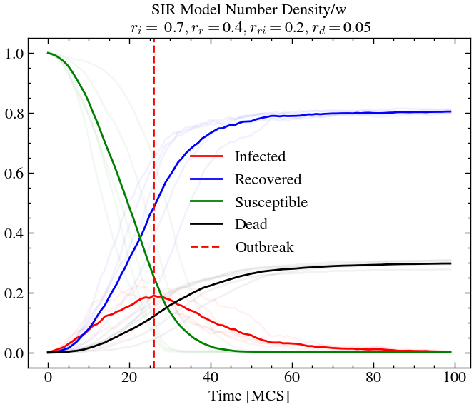
infection_rate, recovery_rate, reinfection_rate, death_rate = 0.7, 0.4, 0.2, 0.05

L,T = 60,100
ntimes = 5
with ProgressBar(total=ntimes) as progress:
    world_evolution_sir, number_densities_sir = run_SIR(ntimes, L, T, species, initial_densities, infection_rate, recovery_rate, reinfection_rate, death_rate, progress)

n_avg = plot_sir(number_densities_sir, infection_rate, recovery_rate, reinfection_rate, death_rate, 0.05)

fig, ax = plt.subplots(figsize=(6,7))

def animate(ti, title):
    ax.clear()
    image = np.zeros((L, L, 3), dtype=np.uint8)
    image[:, :, 0] = 255*(world_evolution_sir[ti, 1]) # R -> infected
    image[:, :, 1] = 255*(world_evolution_sir[ti, 0]) # G -> susceptible
    image[:, :, 2] = 255*(world_evolution_sir[ti, 2]) # B -> recovered
    ax.imshow(image)
    ax.set_title(f'{title}\nMCS = {ti:2}')
    ax.set_xticks([]) 
    ax.set_yticks([]) 
    return fig,

title = 'SIR Model w/\n $r_i =$ ' + str(infection_rate) + '$, r_r=$' + str(recovery_rate) + '$, r_{ri}=$' + str(reinfection_rate) + '$, r_d=$' + str(death_rate)
ani = animation.FuncAnimation(fig, animate, frames=T, interval=50, blit=True, fargs=(title,))
ani.save('animations/SIR2.gif',writer='pillow',fps=20)

HTML(ani.to_html5_video())

Same transmission, lower re-infection rate¶

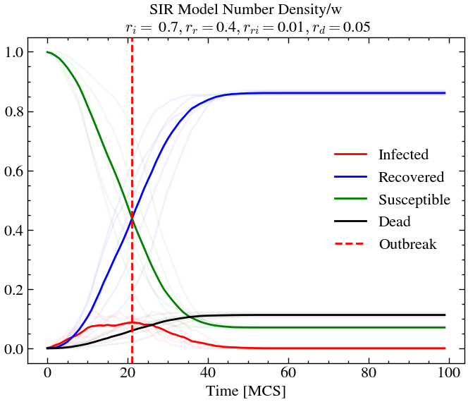
infection_rate, recovery_rate, reinfection_rate, death_rate = 0.7, 0.4, 0.01, 0.05

L,T = 60,100
ntimes = 5
with ProgressBar(total=ntimes) as progress:
    world_evolution_sir, number_densities_sir = run_SIR(ntimes, L, T, species, initial_densities, infection_rate, recovery_rate, reinfection_rate, death_rate, progress)

n_avg = plot_sir(number_densities_sir, infection_rate, recovery_rate, reinfection_rate, death_rate, 0.05)

fig, ax = plt.subplots(figsize=(6,7))

def animate(ti, title):
    ax.clear()
    image = np.zeros((L, L, 3), dtype=np.uint8)
    image[:, :, 0] = 255*(world_evolution_sir[ti, 1]) # R -> infected
    image[:, :, 1] = 255*(world_evolution_sir[ti, 0]) # G -> susceptible
    image[:, :, 2] = 255*(world_evolution_sir[ti, 2]) # B -> recovered
    ax.imshow(image)
    ax.set_title(f'{title}\nMCS = {ti:2}')
    ax.set_xticks([]) 
    ax.set_yticks([]) 
    return fig,

title = 'SIR Model w/\n $r_i =$ ' + str(infection_rate) + '$, r_r=$' + str(recovery_rate) + '$, r_{ri}=$' + str(reinfection_rate) + '$, r_d=$' + str(death_rate)
ani = animation.FuncAnimation(fig, animate, frames=T, interval=50, blit=True, fargs=(title,))
ani.save('animations/SIR3.gif',writer='pillow',fps=20)

HTML(ani.to_html5_video())

Same transmission, zero death rate¶

infection_rate, recovery_rate, reinfection_rate, death_rate = 0.7, 0.4, 0.2, 0.0

L,T = 60,100
ntimes = 5
with ProgressBar(total=ntimes) as progress:
    world_evolution_sir, number_densities_sir = run_SIR(ntimes, L, T, species, initial_densities, infection_rate, recovery_rate, reinfection_rate, death_rate, progress)

n_avg = plot_sir(number_densities_sir, infection_rate, recovery_rate, reinfection_rate, death_rate, 0.05)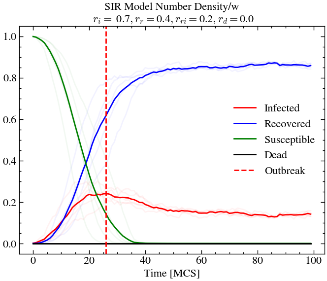

fig, ax = plt.subplots(figsize=(6,7))

def animate(ti, title):
    ax.clear()
    image = np.zeros((L, L, 3), dtype=np.uint8)
    image[:, :, 0] = 255*(world_evolution_sir[ti, 1]) # R -> infected
    image[:, :, 1] = 255*(world_evolution_sir[ti, 0]) # G -> susceptible
    image[:, :, 2] = 255*(world_evolution_sir[ti, 2]) # B -> recovered
    ax.imshow(image)
    ax.set_title(f'{title}\nMCS = {ti:2}')
    ax.set_xticks([]) 
    ax.set_yticks([]) 
    return fig,

title = 'SIR Model w/\n $r_i =$ ' + str(infection_rate) + '$, r_r=$' + str(recovery_rate) + '$, r_{ri}=$' + str(reinfection_rate) + '$, r_d=$' + str(death_rate)
ani = animation.FuncAnimation(fig, animate, frames=T, interval=50, blit=True, fargs=(title,))
ani.save('animations/SIR4.gif',writer='pillow',fps=20)

HTML(ani.to_html5_video())

SIR analysis¶

As evident in the four different simulations we have performed, we can deduce the following.

For low infection rate (or transmission rate), but low recovery rate, we see that individuals are sick for longer times, meaning there is more chance of death, even if the death rate is relatively low. Here, the re-infection rate does not matter since there is lower chance of recovery anyway. At outbreak, we see the only around 10% of the population is infected. However, at later times, around 40% of the population are dead. We see that there is still a non-zero amount of susceptible individuals at later times. This is an unfortunate consequence of the high death rate causing the disease to not reach certain pockets of society where there are only healthy individuals. Hence, this an example of structure formation as well.
For high infection rate and high recovery rate (and high re-infection rate), we see that around 20% of the population is infected at outbreak, but the overall death rate is lower than before. At later times almost the entire population has been infected at-least once or dead. This is not the case for scenario 1, where we see that there is still some amount of susceptible people left at later times.
If we now decrease the re-infection rate (for exmaple, through vaccination drives etc.), keeping everything else constant, we see that less that 10% of the population is infected at outbreak and only around 10% of the total population dies, compared to the previous scenario where around 30% of the population died.
Now, if increase back the re-infection rate, but set the death rate to zero, this, just means that even after outbreak, quite a significant number of people (under 20%) are always infected at a given time. Since there is no possibility of death, the disease just gets passed around forever, and can only be eradicated through lower re-infection rates (aka vaccination, for example).

Conclusion¶

In this project, we haved discussed Markovian agent-based simulations of stochastic models that describe bio-chemical reactions, population dynamics, and epidemic spreading. The underlying assumption of such simulations are that much of a complex system’s features are irrelevant in capturing the essence of its gross dynamical properties.

Using three different types of systems - reaction diffusion models, Lotka-Volterra Prey Predator model and SIR modelling for disease spreading in populations, we have seen that Monte-Carlo methods are quite usefuly in visualising the dynamics of simulations, as well as tracking populations sizes whereas differential equations only tell us about the evolution of quantities like population sizes – which is just a numerical value. Because of this, features like structure formation, and corrlation functions can only be studied using Monte-Carlo simulations. We saw that any quantity of interest should be computed for sufficiently many individual trajectories to ensure that the results are statistically significant and reach the desired accuracy, as the error scales as $\sim (\sqrt{N})^{-1}$ . It is to be noted that sometimes results obtained from Monte-Carlo methods do not always constitute unwanted artefacts, but instead may genuinely reflect model properties which can only be derived stochastically.

However, even though it is conceptually easy to add additional dynamical features to a model system, it becomes impractical to properly run parameter sweeps to adequately assess their characteristic regimes. This ultimately constrains the applicability of stochastic simulation models.

Future Possibilities¶

The authors of this paper have analysed a wide array of possibilies when it comes to using Markovian agent based Monte-Carlo simulations. Since we are dealing with simple particle reactions, and predefined probabilities, the possibilities are endless with what could be done more. Some of them are listed below.

The authors have provided the code for the Lotka-Volterra model, but it is really slow since they have prioritised readability over code efficiency. I have tried to implement a numba based code in this notebook, which uses parallel processing and produces optimized machine code at runtime, which speeds up the simulations by more than 50x (in the case of my computer). They could have implemented a more efficient but still readable, something which uses @jitclass decorator, which is the numba mechanism to optimize python classes.
For the prey-predator models, they could have performed more advanced forms of simulations, wherein we track inherited traits to show Darwinian evolution or use more complex multi-layered ecological dynamics involving more than two species.
For the SIR Modelling, the focus of the paper was on the mathematical evolution and not necessarily the real-world implications of various scenarios as we play around with the parameters. They could have compared this with real world data, for example the COVID-19, since in practical scenarios, parameters like infection, recovery and immunity rates are heavily dependent on time as the world changes rapidly. While this could be outside the scope of this paper, several other works like Mukhamadiarov, R. et. al. (2021) and Chen, K. et. al. (2023) discuss this more in detail.

References¶

Mukhamadiarov, R. I., Deng, S., Serrao, S. R., Priyanka, Nandi, R., Yao, L. H., & Täuber, U. C. (2021). Social distancing and epidemic resurgence in agent-based susceptible-infectious-recovered models. Scientific Reports, 11(1). 10.1038/s41598-020-80162-y
Chen, K., Jiang, X., Li, Y., & Zhou, R. (2023). A stochastic agent-based model to evaluate COVID-19 transmission influenced by human mobility. Nonlinear Dynamics, 111(13), 12639–12655. 10.1007/s11071-023-08489-5